Introduction

Geostatistics provides a robust framework for spatial interpolation and is widely used across environmental science, natural resource management, and mining engineering. The accurate estimation of values over a defined area, or “block,” is a fundamental requirement in these fields, where decisions are often based on aggregate rather than point-specific data. Block kriging (Goovaerts 1997), an extension of the broader kriging technique, is the standard method for this purpose, offering the best linear unbiased prediction of block averages. In this blog post, we will explore the principles of block kriging, its advantages and applications, and how it compares to point kriging. The evaluation will be performed using the R language for statistical computing and visualization and the R package gstat.

Background

Block kriging is a geostatistical method that estimates the average value of a variable over a defined area, or “block,” rather than predicting the value at a single, unsampled point. It is a variant of point kriging, which is typically used for smaller-scale, localized estimations. Block kriging inherently generates smoother maps than point kriging, helping to negate the effects of discontinuities in the data as well as other undesirable artifacts. The block kriging variance is lower in comparison to point kriging because the local scale variation, or within-block variation, is removed, which is an advantage for data sets with a large nugget.

While this can be beneficial for reducing estimation variance, it has some drawbacks. The smoothing effect can obscure the true variability of the data by underestimating high values and overestimating low ones. For instance, in a mining context, this could lead to underestimating the value of high-grade ore blocks, potentially understating a mine’s economic potential. Additionally, the fine-scale details and extreme values present in the original data may be lost by averaging over a block. However, block kriging can be very useful for those instances where there is little interest in predicting a value at a specific location, but instead the focus is on the value over a larger spatial support, such as exposure units for soil pollution, management units in agriculture, or blocks for mining.

Preliminaries

We’ll start by loading the main R libraries that will be used for loading and processing the data, and for performing ordinary point and block kriging.

# Load libraries
library(dplyr)
library(sf)
library(gstat)
library(ggplot2)
library(stars)
library(geostatsp)

Let’s set the European Petroleum Survey Group (EPSG) code for our data. The EPSG code is a unique identifier for different coordinate systems. It’s a public registry of geodetic datums, spatial reference systems, Earth ellipsoids, coordinate transformations, and related units of measurement. Switzerland primarily uses the Universal Transverse Mercator (UTM) system, specifically UTM zone 32N, often referenced with the WGS 84 geodetic datum.

# Set EPSG code
epsg <- 32632   # WGS 84, UTM Zone 32N (meters)

Data

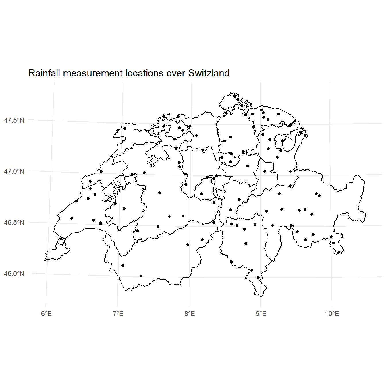
The data consist of 100 daily rainfall measurements made in Switzerland on the 8th of May 1986. These data represent a subset of the original data, randomly sampled for use in a 1997 spatial interpolation comparison study (Dubois et al. 2003). The data are available in the R package geostats. A shapefile of the 26 cantons of Switzerland will be used as part of the analysis. The 26 cantons of Switzerland are the member states of the Swiss Confederation.

# Load the data
data('swissRain')
swissRain <- unwrap(swissRain)

# Load a shapefile for the Swiss cantons
ch <- read_sf('swisscantons/ch-cantons.shp')

Let’s convert the rainfall data into a sf object with the appropriate UTM projection system for Switzerland using the EPSG code. Let’s also convert the shapefile of the 26 cantons of Switzerland to the same projecton system.

# Convert data into a sf object with appropriate UTM projection
crs <- st_crs(paste0('EPSG:', epsg))
swissRain.sf <- st_as_sf(swissRain) %>%
 st_transform(crs)

# Convert shapefile appropriate UTM projection
ch <- st_transform(ch, crs)

Below is a map of the 26 cantons of Switzerland showing the locations of the 100 daily rainfall measurements.

# Plot data
ggplot() +
  geom_sf(data = st_cast(ch, 'MULTILINESTRING')) + 
  geom_sf(data = swissRain.sf) +
  labs(title = 'Rainfall measurement locations over Switzland',
       x = NULL,
       y = NULL) +
  theme_minimal()

Variogram

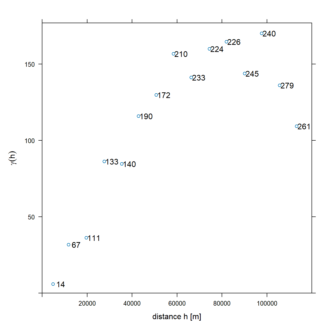
Kriging requires a model of spatial correlation. Spatial autocorrelation can be modeled using the variogram or covariance function. Typically, the sample variogram is plotted based on the data, and a variogram model is fit to the sample variogram. The variogram is a quantitative descriptive statistic that can be graphically represented in a manner which characterizes the spatial continuity of a data set.

Let’s compute and plot the sample variogram of the rainfall data. The variogram() function in the R package gstat chooses as default one-third the length of the bounding box diagonal for maximum distance (cutoff) and the cutoff divided by 15 for interval width (width).

# Compute  and plot variogram
v <- variogram(rain ~ 1, data = swissRain.sf)
plot(
  v, plot.numbers = TRUE,
  xlab = 'distance h [m]',
  ylab = expression(gamma(h)),
  xlim = c(0, 1.06 * max(v$dist))
)

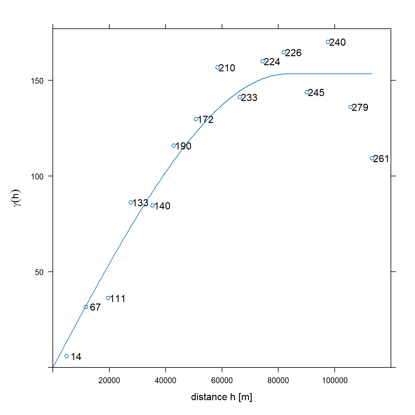
The fitted variogram model is used to calculate the data values at each modeled point. Therefore, a model must be created that is as representative as possible of the spatial characteristics of the data set and, by extension, of the sample variogram.

Let?s fit an omnidirectional spherical variogram model to the rainfall data using the fit.variogram() function in the R package gstat. The fitting method uses nonlinear regression to fit the coefficients using weighted sum-of-square errors (Bivand et al. 2013).

# Fit variogram by weighted least squares (WLS)
v.m <- fit.variogram(v, vgm(1, 'Sph', 50000, 1))
plot(
  v, v.m, plot.numbers = TRUE,
  xlab = 'distance h [m]',
  ylab = expression(gamma(h)),
  xlim = c(0, 1.06 * max(v$dist))
)

Kriging

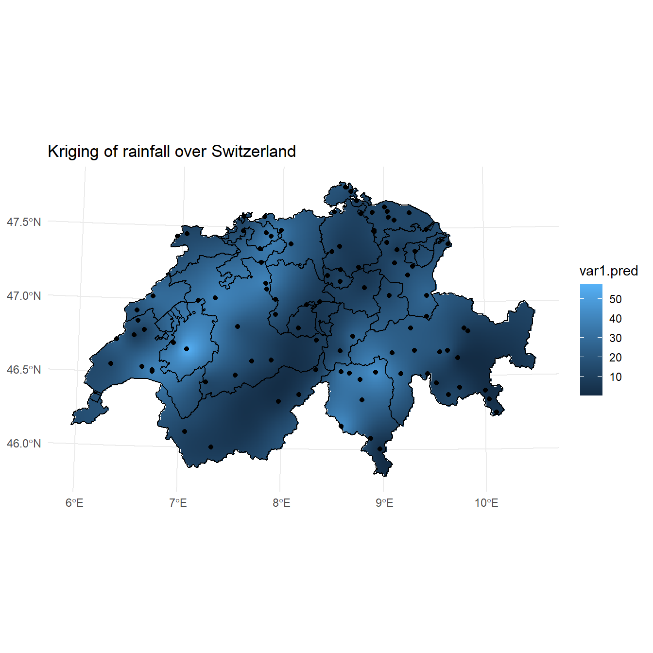
Ordinary kriging assumes that the overall mean is constant, though unknown, and the variance is finite (the variogram has a sill value). The goal is to produce a set of estimates for which the variance of the errors is minimized. To accomplish this goal, ordinary kriging weights each sample based on its relative distance from the location of the data point to be predicted.

First, well will create a regular 1 km x 1 km grid covering Switzerland using the shapefile object. Then we will use this grid to perform ordinary kriging of the rainfall data using the krige() function in the R package gstat. A plot of the kriging predictions is shown below.

# Create a regular 1 km x 1 km grid covering Switzerland using the object ch
grd <- st_bbox(ch) %>%
  st_as_stars(dx = 1000) %>%
  st_crop(ch)
grd
## stars object with 2 dimensions and 1 attribute
## attribute(s):
##         Min. 1st Qu. Median Mean 3rd Qu. Max.  NA's
## values     0       0      0    0       0    0 36790
## dimension(s):
##   from  to  offset delta                refsys x/y
## x    1 350  264867  1000 WGS 84 / UTM zone 32N [x]
## y    1 223 5295762 -1000 WGS 84 / UTM zone 32N [y]

# Perform ordinary kriging
kr <- krige(rain ~ 1, swissRain.sf, grd, model = v.m)
## [using ordinary kriging]

# Plot kriging results
ggplot() +
  geom_stars(data = kr, aes(x = x, y = y, fill = var1.pred),
             na.action = na.omit) + 
  geom_sf(data = st_cast(ch, 'MULTILINESTRING')) + 
  geom_sf(data = swissRain.sf) +
  coord_sf(lims_method = 'geometry_bbox') +
  labs(title = 'Kriging of rainfall over Switzerland',
       x = NULL,
       y = NULL) +
  theme_minimal()

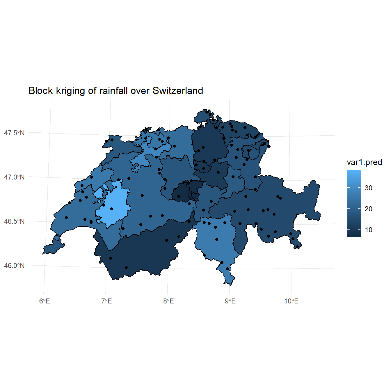
Now, let’s perform block kriging. With the krige() function, this can be done by giving the target areas (polygons of the 26 cantons) as the newdata argument. A plot of the block kriging predictions is shown below.

# Perform ordinary kriging
bkr <- krige(rain ~ 1, swissRain.sf, ch, model = v.m)
## [using ordinary kriging]

# Plot kriging results
ggplot() +
  geom_stars(data = st_as_stars(bkr), aes(x = x, y = y, fill = var1.pred)) + 
  geom_sf(data = st_cast(ch, 'MULTILINESTRING')) + 
  geom_sf(data = swissRain.sf) +
  coord_sf(lims_method = 'geometry_bbox') +
  labs(title = 'Block kriging of rainfall over Switzerland',
       x = NULL,
       y = NULL) +
  theme_minimal()

Areal Means

Let’s compute the areal means of the rainfall data by taking the average of the point samples falling inside the target polygons.

# Calculate areal means
amean <- aggregate(swissRain.sf['rain'], by = ch, FUN = mean)

Let’s combine the simple averaging of the point samples with the areal means from the block kriging and plot the results of both methods.

# Merge the two data sets into a single object
bkr$sample <- amean$rain
bkr$kriging <- bkr$var1.pred
pred <- bkr %>%
  dplyr::select(sample, kriging) %>% 
  tidyr::pivot_longer(1:2, names_to = 'var', values_to = 'rain')
pred$var <- factor(pred$var, levels = c('sample', 'kriging'))

# Plot the results
ggplot() +
  geom_sf(data = pred, mapping = aes(fill = rain)) +
  facet_wrap(~var, ncol = 1) +
  labs(title = paste0(
    'Aggregated rainfall from simple averaging (top) and\n',
    'block kriging (bottom)')
  ) +
  scale_fill_gradientn(colors = sf.colors(20)) +
  theme_minimal()

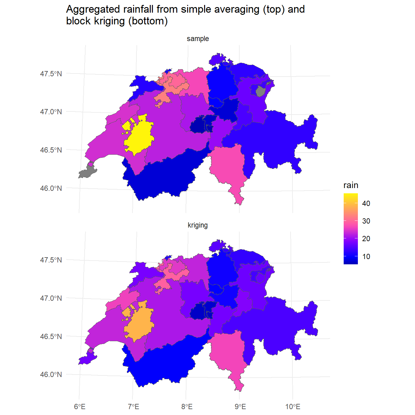
The plots look similar, although the sample means from the block kriging appear to exhibit less variability than simple averaging.

Standard Errors

Now, let’s compare the standard errors of means for the two methods. For the simple averaging,
the standard error can be approximated by \(\sqrt{\sigma^2/n}\). The block kriging variance is the model-based estimate and is a by-product of the kriging process.

SE <- function(x) sqrt(var(x)/length(x))
aerr <- aggregate(swissRain.sf['rain'], ch, SE)

# Merge the two data sets into a single object
bkr$sample <- aerr$rain
bkr$kriging <- sqrt(bkr$var1.var)
pred <- bkr %>%
  dplyr::select(sample, kriging) %>% 
  tidyr::pivot_longer(1:2, names_to = 'var', values_to = 'error')
pred$var <- factor(pred$var, levels = c('sample', 'kriging'))

# Compare the simple averaging approach to block kriging
ggplot() +
  geom_sf(data = pred, mapping = aes(fill = error)) +
  facet_wrap(~var, ncol = 1) +
  labs(title = paste0(
    'Standard errors for mean rainfall obtained by simple\n',
    'averaging (top) and block kriging (bottom)')
  ) +
  scale_fill_gradientn(colors = sf.colors(20)) +
  theme_minimal()

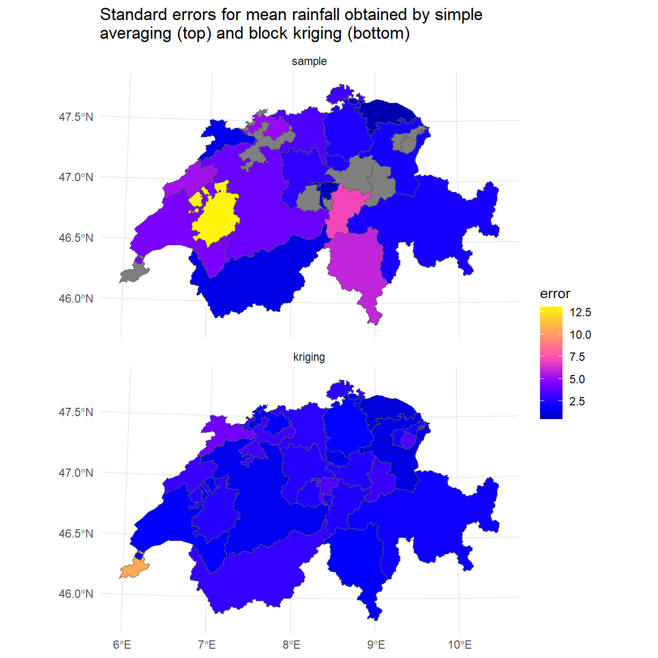
We see that the simple averaging approach exhibits more variability and larger values of the areal mean prediction errors than that of block kriging. By averaging over a block, the impact of measurement errors associated with individual point measurements is reduced.

Conclusion

Block kriging is a geostatistical method that, by estimating average values over defined areas rather than at discrete points, produces smoother maps and lower estimation variance than point kriging,as demonstrated through the analysis of daily rainfall measurements in Switzerland. Despite potentially obscuring true data variability, block kriging is valuable when the focus is on values over larger spatial supports, ultimately yielding less variable and more accurate areal mean predictions compared to simple averaging.

References

Bivand, R.S., E. Pebesma, and V. Gomez-Rubio. 2013. Applied Spatial Data Analysis with R, Second Edition. Springer, New York.

Dubois, G., Malczewski, J. and De Cort, M. (2003). Mapping radioactivity in the environment. Spatial Interpolation Comparison 97 (Eds.). EUR 20667 EN, EC.

Goovaerts, P.. 1997. Geostatistics for Natural Resources Evaluation. Oxford Univiversity Press, New York.