Introduction

On January 28, 1986 the space shuttle Challenger disintegrated 73 seconds after liftoff from Kennedy Space Center. The disaster claimed the lives of all seven astronauts aboard, including Christa McAuliffe, a teacher from New Hampshire who would have been the first civilian in space. There are many lessons to be learned from this tragedy. The accident illustrates the potentially disastrous consequences of poor organizational culture, illustrating the need for proper organizational structure. It also shows how group think can have dire consequences. Edward Tufte, a well-known statistician and data visualization expert presents the tragedy in a different perspective. He argues that not having the data presented in an easily readable format led to the tragedy as well. Let’s examine how statistical science could have provided valuable input to the launch decision process.

Background

Immediately after the tragedy, the Presidential Commission on the Space Shuttle Challenger Accident (also known as the Roger’s Commission) was established to ascertain the cause of the accident. They found that the immediate cause of the accident was the failure of a key structural component of the shuttle’s rockets. Two rubber O-rings, which had been designed to separate the sections of the rocket booster, had failed due to cold temperatures on the morning of the launch. Rocket fuel exploded after escaping through an opening left by a failed O-ring. The Commission further noted that there were organizational problems with NASA that contributed to the catastrophe.

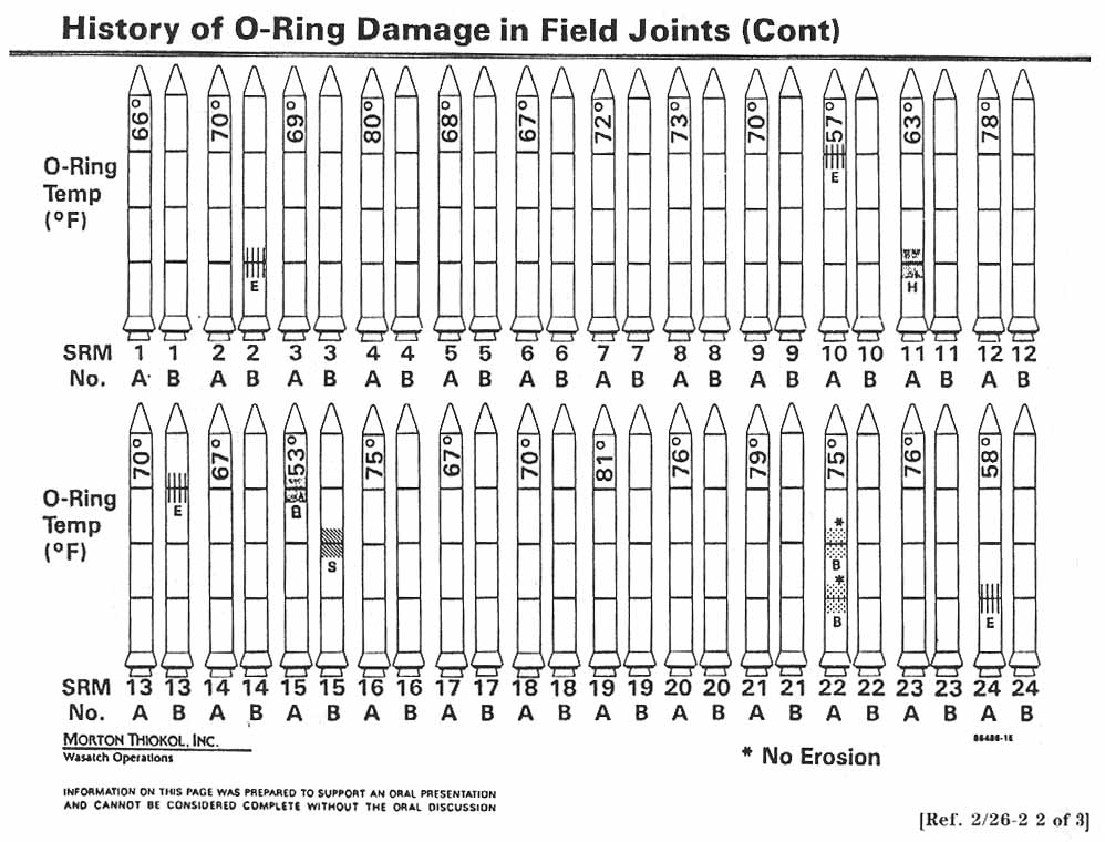
On the afternoon of January 27, 1986, the eve of the launch, the weather forecast predicted unusually cold weather for Florida during the early hours of January 28. Engineers of the booster rockets’ manufacturer expressed concern that at cold temperatures, the O-rings would harden and not seal the joints against the hot ignition gases. Rocket tests had previously shown evidence of thermal stress in O-rings when temperatures were 65°F and colder; no data were available for the low temperatures predicted for launch time. Charts displaying outlines of rockets labelled with temperatures of O-ring damage, organized by launch date were presented to NASA.

Faxes sent to NASA on January 27th, the night before the launch, presented a graph of damage incidents to one or more rocket O-rings as a function of temperature.

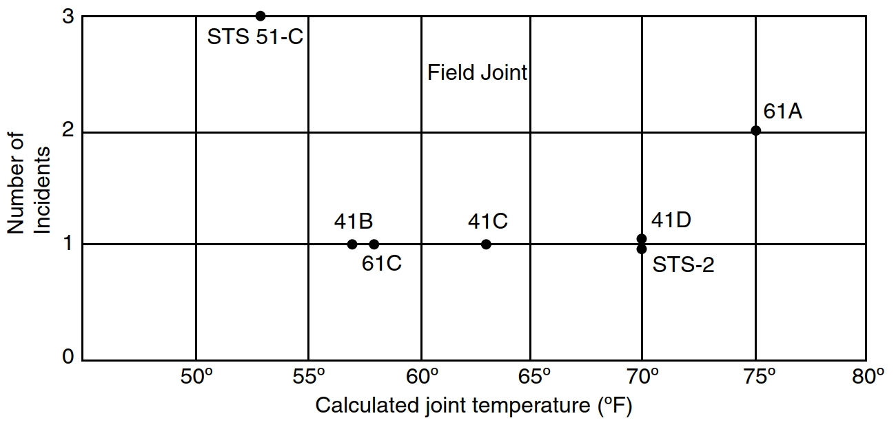
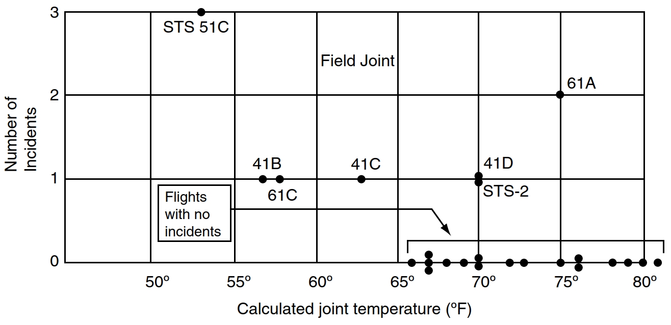
Evidence given in the figure seemed inconclusive to NASA managers. There were few data and what data were available, did not show a clear relationship between temperature and the number of O-ring failures. However, as noted by the Roger’s Commission, the graph had one major flaw-flights where damage had not been detected were deleted. The Commission produced a modified graph, were they added back in the censored values. By including all recorded data, the Commission indicated that the pattern was a bit more striking.

What Analysis Could Have Been Performed?

The vast amount of information in censored observations is contained in the proportions at which they occur. A simple bar chart could have focused on the proportion of O-rings exhibiting damage. For a possible total of three damage incidents in each rocket, a graph of the proportion of failure incidents by temperature range would have illustrated an increase in the proportion of damaged O-rings with lower temperatures.

Alternatively, we might be interested in modelling the effect of treatment on the probability of O-ring failure. We can do this by fitting a binomial linear logistic model. A statistical model appropriate for this data, conditional on temperature, t, is the binomial model. There are six O-rings on the shuttle, so during each launch, the number of distress events, is modeled as binomial with parameters p = p(t) and n = 6. The model assumes that at temperature t each of the six O-rings would suffer damage independently with the same probability. To link p(t) to t, a logistic regression model is used:

$$Log[\frac{p(t)}{(1-p(t)}] = \alpha + \beta \cdot t$$

R makes it very easy to fit a logistic regression model. The function to be called is glm() and the fitting process is not so different from the one used in linear regression as shown below.

library(vcd)
data(SpaceShuttle)
failed <- SpaceShuttle[with(SpaceShuttle, Fail == 'yes'),]
nofailed <- SpaceShuttle[with(SpaceShuttle, Fail == 'no'),]
fm <- glm(
  cbind(nFailures, 6 - nFailures) ~ Temperature,
  data = SpaceShuttle,
  family = binomial
)
fm

## 
## Call:  glm(formula = cbind(nFailures, 6 - nFailures) ~ Temperature, 
##     family = binomial, data = SpaceShuttle)
## 
## Coefficients:
## (Intercept)  Temperature  
##      5.0850      -0.1156  
## 
## Degrees of Freedom: 22 Total (i.e. Null);  21 Residual
##   (1 observation deleted due to missingness)
## Null Deviance:	    24.23 
## Residual Deviance: 18.09 	AIC: 35.65

The estimates of the coefficients are \(\alpha\) = 5.085 and \(\beta\) = -0.1156. Using the regression model, it’s a simple exercise to create a graph presenting the probability of O-ring failure as a function of temperature.

plot(nFailures/6 ~ Temperature, data = failed,
     xlim = c(30, 81), ylim = c(0, 1),
     main = 'NASA Space Shuttle O-Ring Failures',
     xlab = 'Temperature (F)',
     ylab = 'Estimated Failure Probability',
     pch = 19, cex = 1.2, col = 4)
abline(v = 31, lwd = 3, lty = 3)
points(nFailures/6 ~ Temperature, data = nofailed, pch = 19, cex = 1.2, col = 4)
lines(
  30:81, predict(fm, data.frame(Temperature = 30 : 81), type = 're'),
  lwd = 2
)
pr <- predict(fm, data.frame(Temperature = 30:81), se = T)
upper <- pr$fit + 1.96*pr$se.fit
lower <- pr$fit - 1.96*pr$se.fit
lines(30:81, plogis(upper), lwd = 3, lty = 3, col = 2)
lines(30:81, plogis(lower), lwd = 3, lty = 3, col = 2)

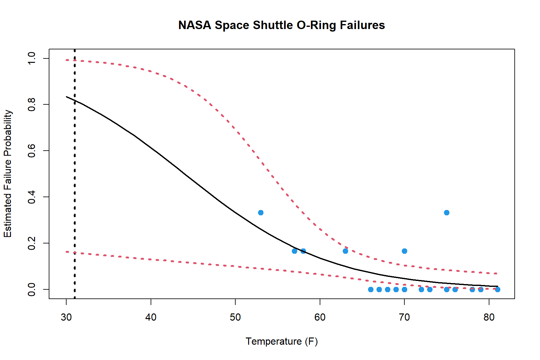
Approximate 95% confidence intervals based on asymptotic normality are included to assess the reliability of the results. Bootstrap confidence intervals could be used instead of using the asymptotic theory to construct confidence intervals, but we’ll leave that for another day. Notice that the intervals are wide for temperatures less than 60°F and narrow for temperatures greater than 60°F. This is expected because most of the data have temperatures greater than 60°F. The estimated probability interval at 31°F, the anticipated temperature of launch, illustrates the high variability in the expected number of failures at this low temperature.

Conclusions

The most disturbing part of the space shuttle Challenger disaster was that the O-ring failure had been foreseen by the manufacturer’s engineers, who were unable to convince managers to delay the launch. Providing a better analysis and visualization of the data could have helped improve the decision-making process and potentially built a stronger case for the engineers about the effect of cold weather on O-ring functionality.