Insider Censoring in Environmental Data: Why It Biases Results and How to Fix It
By Charles Holbert
March 15, 2026
Introduction
Environmental datasets frequently include measurements reported near analytical detection and quantitation or reporting limits. Although these limits are inherent features of laboratory analysis, the reporting conventions applied to them can materially influence the conclusions drawn from the data. One particularly problematic practice is insider censoring, which occurs when the censoring threshold depends on the measured value itself. This creates a form of informative censoring that violates a fundamental assumption of censored-data methods—that censoring remain noninformative with respect to the underlying concentrations. As a result, insider censoring is not merely a statistical technicality; it is a data preprocessing practice that can structurally alter environmental datasets and potentially influence regulatory conclusions.
This post examines insider censoring, explains why it introduces bias in environmental datasets, and discusses approaches for mitigating its effects. It demonstrates the issue with a simulated example, illustrating how different censoring schemes affect reported concentrations, distributional shape, and summary statistics. The post concludes by emphasizing the importance of proper data management practices when working with censored environmental datasets. The calculations are performed using R version 4.4.3 (R Core Team 2026).
Background
Environmental measurements are commonly reported relative to analytical detection limits. The Method Detection Limit (DL) represents the lowest concentration distinguishable from zero, while the Reporting or Quantitation Limit (RL/QL) represents the lowest concentration that can be reliably quantified. Results above the RL are reported as detected values, concentrations between the DL and RL are often reported as J-qualified estimates, and values below the DL are reported as U-qualified nondetects.
Insider censoring occurs when nondetect observations are censored at the higher RL while detected values remain below that threshold (Helsel 2005; 2012). This situation commonly arises when nondetect results are substituted with the reporting limit during data preprocessing while J-qualified measurements between the DL and RL are retained as numeric values. The resulting dataset is internally inconsistent and violates the assumption of noninformative censoring required by standard censored-data methods.
This practice artificially elevates low observations, distorting summary statistics, regression results, and the apparent shape of the data distribution. Such distortions can influence modeling, hypothesis testing, and environmental risk assessments in which small concentration differences may affect regulatory or exposure decisions.
The issue is not the existence of detection limits—which are unavoidable—but how measurements near those limits are reported and analyzed. When reporting conventions obscure the distinction between nondetects and uncertain detects, structural bias may be introduced into the dataset. Consistent reporting thresholds and appropriate statistical treatment of censored data are therefore necessary to ensure that environmental datasets accurately represent the underlying measurements and support reliable scientific conclusions.
Identification of Insider Censoring
Detecting insider censoring requires careful examination of both the reported data and the laboratory reporting practices used to produce the dataset. Several signs may indicate its presence.
One indicator is multiple RLs within the dataset, particularly when nondetect values are consistently reported at a higher threshold than some measured concentrations. For instance, if numeric results appear below a stated RL or QL, it may suggest that the laboratory measured concentrations below that threshold but applied a higher RL when reporting nondetects. Another sign is the clustering of censored observations at an RL that is higher than the lowest measured value in the dataset. In these cases, the reported RL may not represent the method’s actual detection capability.
Reviewing laboratory documentation can help identify insider censoring. Reports often list detection, reporting, and quantitation limits separately; when these limits differ, analysts should evaluate how each one is applied in the dataset. Finally, graphical inspection of the data can reveal suspicious patterns. Histograms or cumulative distribution plots may show an artificial buildup of observations at the RL that is inconsistent with the distribution of measured values.
Simulation
To illustrate the practical consequences of insider censoring, the following simulation compares several common approaches for handling observations near detection and reporting limits.
Simulated Data
In this simulation, 100 lognormal concentrations with a lognormal mean of 1 and a standard deviation of 0.5 are generated. The DL and RL are chosen to make the censoring patterns easy to visualize. The underlying data are then represented in four different ways. The first treats all observations as detected values. The second uses a stepped approach, where U-qualified results are censored at the DL and J-qualified values remain between the DL and RL. The third applies insider censoring, in which U-qualified results are censored at the RL while J-qualified values are still reported below it. The fourth shows an alternative approach that assigns the RL to both U- and J-qualified values that fall below the RL.
suppressPackageStartupMessages({
  library(dplyr)
  library(ggplot2)
  library(NADA)
  library(EnvStats)
})

# Load local helper functions used by the UCL workflow
source('functions/ucls.R')

# Set seed
set.seed(123)

# Simulated parameters
n <- 100
true_meanlog <- 1
true_sdlog <- 0.5
DL <- 1.5
RL  <- 3

# Generate true lognormal concentrations
x_true <- rlnorm(n, meanlog = true_meanlog, sdlog = true_sdlog)

# Helper to create each method
create_method <- function(values, method, DL, RL) {
  qualifier <- rep("Detect", length(values))
  reported  <- values

  if (method == "100% detects") {
    qualifier <- rep("Detect", length(values))
  }

  if (method == "Stepped") {
    reported[values < DL] <- DL
    qualifier[values < DL] <- "U"
    qualifier[values >= DL & values < RL] <- "J"
  }

  if (method == "Insider") {
    reported[values < DL] <- RL
    qualifier[values < DL] <- "U"
    qualifier[values >= DL & values < RL] <- "J"
  }

  if (method == "Alternative") {
    reported[values < RL] <- RL
    qualifier[values < RL] <- "U"
  }

  data.frame(
    Method = method,
    true_value = values,
    reported_value = reported,
    qualifier = qualifier,
    stringsAsFactors = FALSE
  )
}

# Build combined dataset
df_detect <- create_method(x_true, "100% detects", DL, RL)
df_step   <- create_method(x_true, "Stepped", DL, RL)
df_inside <- create_method(x_true, "Insider", DL, RL)
df_alt    <- create_method(x_true, "Alternative", DL, RL)

plot_df <- rbind(df_detect, df_step, df_inside, df_alt)

plot_df$Method <- factor(
  plot_df$Method,
  levels = c("100% detects", "Stepped", "Insider", "Alternative")
)

plot_df$qualifier <- factor(
  plot_df$qualifier,
  levels = c("Detect", "J", "U")
)
How Insider Censoring Changes the Data
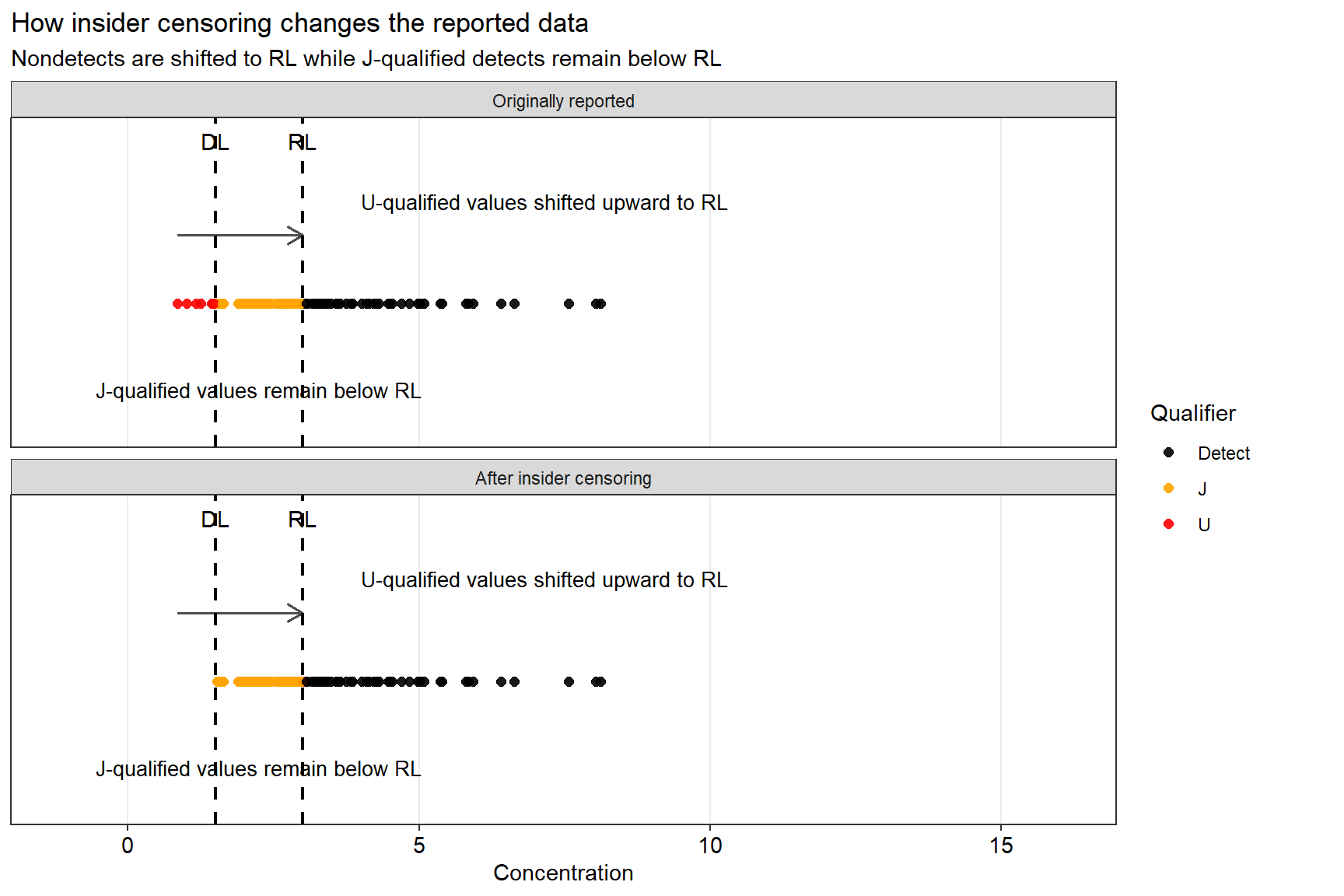
The plot below shows how insider censoring changes the data. Values below the DL are shifted upward to the RL, but J-qualified values remain below that same RL. This creates a lower tail that is no longer internally consistent.
# Pull the Insider method data from the existing simulation
insider_vis <- plot_df %>%
  filter(Method == "Insider") %>%
  mutate(
    original_x = true_value,
    shifted_x  = reported_value
  )

# Build two panels:
# 1) Originally reported = true simulated values with qualifiers
# 2) After insider censoring = reported values used in analysis
before_df <- insider_vis %>%
  transmute(
    stage = "Originally reported",
    x = original_x,
    qualifier = as.character(case_when(
      original_x < DL ~ "U",
      original_x < RL  ~ "J",
      TRUE             ~ "Detect"
    ))
  )

after_df <- insider_vis %>%
  transmute(
    stage = "After insider censoring",
    x = shifted_x,
    qualifier = as.character(qualifier)
  )

# Arrows only for U-qualified points that were shifted upward to RL
arrow_df <- insider_vis %>%
  filter(true_value < DL) %>%
  transmute(
    x = true_value,
    xend = reported_value,
    y = 1.08,
    yend = 1.08
  )

plot_df2 <- bind_rows(before_df, after_df)

plot_df2$stage <- factor(
  plot_df2$stage,
  levels = c("Originally reported", "After insider censoring")
)

plot_df2$qualifier <- factor(
  plot_df2$qualifier,
  levels = c("Detect", "J", "U")
)

ggplot(plot_df2, aes(x = x, y = 1, color = qualifier)) +
  geom_point(size = 2, alpha = 0.9) +
  geom_segment(
    data = arrow_df,
    aes(x = x, xend = xend, y = y, yend = yend),
    inherit.aes = FALSE,
    arrow = arrow(length = unit(0.12, "inches")),
    linewidth = 0.7,
    color = "gray30"
  ) +
  geom_vline(xintercept = DL, linetype = "dashed", linewidth = 0.8) +
  geom_vline(xintercept = RL,  linetype = "dashed", linewidth = 0.8) +
  annotate("text", x = DL, y = 1.18, label = "DL", vjust = 0) +
  annotate("text", x = RL,  y = 1.18, label = "RL",  vjust = 0) +
  annotate(
    "text",
    x = RL + 1,
    y = 1.12,
    label = "U-qualified values shifted upward to RL",
    hjust = 0,
    size = 3.5
  ) +
  annotate(
    "text",
    x = (DL + RL) / 2,
    y = 0.9,
    label = "J-qualified values remain below RL",
    size = 3.5
  ) +
  facet_wrap(~ stage, ncol = 1) +
  scale_color_manual(
    values = c(
      "Detect" = "black",
      "J" = "orange",
      "U" = "red"
    )
  ) +
  coord_cartesian(
    xlim = c(min(plot_df$true_value) - 2, max(plot_df$reported_value) + 8),
    ylim = c(0.85, 1.2),
    clip = "off"
  ) +
  labs(
    title = "How insider censoring changes the reported data",
    subtitle = "Nondetects are shifted to RL while J-qualified detects remain below RL",
    x = "Concentration",
    y = NULL,
    color = "Qualifier"
  ) +
  theme_bw() +
  theme(
    axis.title.x = element_text(size = 11, color = 'black'),
    axis.text.x = element_text(size = 11, color = 'black'),
    axis.text.y = element_blank(),
    axis.ticks.y = element_blank(),
    panel.grid.major.y = element_blank(),
    panel.grid.minor = element_blank(),
    legend.position = "right",
    plot.margin = margin(5.5, 40, 5.5, 5.5)
  )
What Happens to the Distribution
Insider censoring affects more than summary statistics—it can also alter the apparent shape of the data distribution. This is important because analysts typically examine the distribution first when deciding which statistical methods, transformations, or models to apply.
The plots below compare a standard censored dataset with an insider-censored representation using robust regression on order statistics (ROS) probability plots. ROS is a semi-parametric method commonly used to estimate summary statistics for environmental datasets containing nondetects. In these plots, detected observations are plotted against their theoretical probabilities (quantiles) under a lognormal distribution. A linear regression line is then fitted to these points and used to estimate (impute) values for the nondetect observations.
# Scenario A: Unbiased Censoring (Censored at DL = 2)
obs_unbiased <- x_true
cens_unbiased <- x_true < DL

# Scenario B: Insider Censoring (Values <2 reported as <4)
obs_insider <- x_true
cens_insider <- rep(FALSE, n)

for (i in 1:n) {
  if (x_true[i] < DL) {
    obs_insider[i] <- RL      # Reported as <4
    cens_insider[i] <- TRUE
  } else {
    obs_insider[i] <- x_true[i]
    cens_insider[i] <- FALSE
  }
}

# Create ROS Objects and Plot
res_unbiased <- ros(obs_unbiased, cens_unbiased)
res_insider <- ros(obs_insider, cens_insider)

# Setup plotting area
par(mfrow = c(1, 2))
original_par <- par(no.readonly = TRUE)
par(mar = c(5.1, 4.1, 8, 2.1))

# Plot A: Unbiased
plot(res_unbiased)
mtext("Unbiased (DL = 1.5)", side = 3, line = 4.2, font = 1, cex = 1)

# Plot B: Insider Censoring
plot(res_insider)
mtext("Insider Censored (<1.5 as <3)", side = 3, line = 4.2, font = 1, cex = 1)

# Reset plotting area
par(mfrow = c(1, 1))
par(original_par)
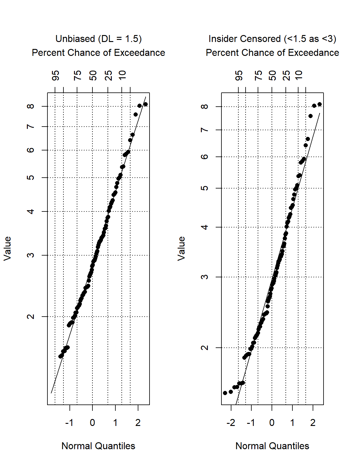
In the unbiased case, the lower tail remains consistent with the overall data pattern. Under insider censoring, however, the lower portion of the probability plot bends because the observations have been redistributed in a way that no longer reflects the original data-generating process.
Comparing Descriptive Statistics Across Methods
Descriptive statistics were compared for the simulated dataset under the four different reporting conventions. Summary statistics include the mean, standard deviation, and a 95% upper confidence limit (UCL) of the mean using censored-data methods. The code below estimates the censored mean and standard deviation using the enparCensored() function in the EnvStats library (Millard 2013) and reports a simple comparative table. The goal is to show the directional effect of the reporting choice.
methods <- levels(plot_df$Method)

results <- plot_df %>%
  mutate(censored = ifelse(qualifier == 'U', 1, 0)) %>%
  group_by(Method) %>%
  summarize(
    Mean = tryCatch(
      ifelse (packageVersion('EnvStats') >= '3.0.0',
        enparCensored(reported_value, censored, restricted = TRUE)$parameters['mean'],
        enparCensored(reported_value, censored)$parameters['mean']
      ),
      error = function(e) mean(reported_value, na.rm = T)
    ),
    SD = tryCatch(
      ifelse (packageVersion('EnvStats') >= '3.0.0',
        enparCensored(reported_value, censored, restricted = TRUE)$parameters['sd'],
        enparCensored(reported_value, censored)$parameters['sd']
      ),
      error = function(e) sd(reported_value, na.rm = T)
    ),
    LOG.SD = tryCatch(
      ifelse (packageVersion('EnvStats') >= '3.0.0',
        enparCensored(log(reported_value), censored, restricted = TRUE)$parameters['sd'],
        enparCensored(log(reported_value), censored)$parameters['sd']
      ),
      error = function(e) sd(log(reported_value), na.rm = T)
    ),
    UCL.NORM = tryCatch(
      ucl_norm(x = reported_value, cen = censored),
      error = function(e) NA
    ),
    UCL.GAMMA = tryCatch(
      ucl_gamma(x = reported_value, cen = censored),
      error = function(e) NA
    ),
    UCL.LNORM = tryCatch(
      ucl_lnorm(x = reported_value, cen = censored),
      error = function(e) NA
    ),
    UCL.NP = tryCatch(
      ucl_nonpar(x = reported_value, cen = censored),
      error = function(e) NA
    ),
    DIST = get_dist(x = reported_value, cen = censored),
    UCL95 = ifelse(DIST == 'Normal', UCL.NORM,
      ifelse(DIST == 'Gamma', UCL.GAMMA,
        ifelse(DIST == 'Lognormal' & LOG.SD < 2, UCL.LNORM, UCL.NP
        )
      )
    ),
    .groups = "drop"
  ) %>%
  dplyr::select(-LOG.SD)
  data.frame()
## data frame with 0 columns and 0 rows

results[] <- lapply(results, function(x) if(is.numeric(x)) signif(x,3) else x)
results  %>%
  knitr::kable(
    align = 'lccccccccc'
  ) %>%
  kableExtra::kable_classic_2(
    full_width = F, position = 'center', html_font = 'Cambria', font_size = 14
  )
| Method | Mean | SD | UCL.NORM | UCL.GAMMA | UCL.LNORM | UCL.NP | DIST | UCL95 |
|---|---|---|---|---|---|---|---|---|
| 100% detects | 3.15 | 1.51 | 3.41 | 3.40 | 3.42 | 3.42 | Gamma | 3.40 |
| Stepped | 3.17 | 1.48 | 3.42 | 3.44 | 3.41 | 3.44 | Lognormal | 3.41 |
| Insider | 3.23 | 1.44 | 3.47 | 3.48 | 3.45 | 3.49 | Lognormal | 3.45 |
| Alternative | 3.64 | 1.14 | 3.83 | 3.84 | 3.79 | 3.85 | Gamma | 3.84 |
The results show that insider censoring increases the estimated 95% UCL relative to methods that apply a consistent censoring threshold, indicating an upward bias introduced by mixed censoring levels. The alternative approach, which assigns the RL to both nondetects and J-qualified results below the RL, maintains internal consistency but produces even larger UCL estimates because more observations are elevated to the RL.
These differences are more easily visualized in the figure below, which compares the distribution of reported concentrations and the resulting 95% UCL estimates across the four reporting methods.
# UCL labels for plotting
y_top <- max(plot_df$reported_value) + 0.5

ucl_labels <- data.frame(
  Method = factor(methods, levels = methods),
  y = y_top,
  label = paste0("95 UCL = ", signif(results$UCL95, 3))
)

# Plot
ggplot(plot_df, aes(x = Method, y = reported_value)) +
  geom_boxplot(outlier.shape = NA, color = "black") +
  geom_jitter(aes(color = qualifier), width = 0.12, height = 0, size = 2, alpha = 0.85) +
  geom_hline(yintercept = DL, linetype = "dashed", linewidth = 0.7) +
  geom_hline(yintercept = RL,  linetype = "dashed", linewidth = 0.7) +
  geom_text(
    data = ucl_labels,
    aes(x = Method, y = y, label = label),
    inherit.aes = FALSE,
    size = 3.7
  ) +
  annotate("text", x = 4.35, y = DL, label = "DL", hjust = 0, size = 4) +
  annotate("text", x = 4.35, y = RL,  label = "RL",  hjust = 0, size = 4) +
  scale_color_manual(
    values = c(
      "Detect" = "black",
      "J" = "orange",
      "U" = "red"
    )
  ) +
  coord_cartesian(ylim = c(min(plot_df$reported_value) - 0.5, y_top + 0.5), clip = "off") +
  labs(
    title = "How are 95% UCLs affected by censoring levels?",
    subtitle = "In the Insider method, J-qualified detects fall below the U censoring level (RL)",
    x = "",
    y = "Simulated concentration",
    color = "Qualifier"
  ) +
  theme_bw() +
  theme(
    axis.title = element_text(size = 12, color = 'black'),
    axis.text = element_text(size = 12, color = 'black'),
    plot.margin = margin(5.5, 40, 5.5, 5.5),
    legend.position = "right"
  )
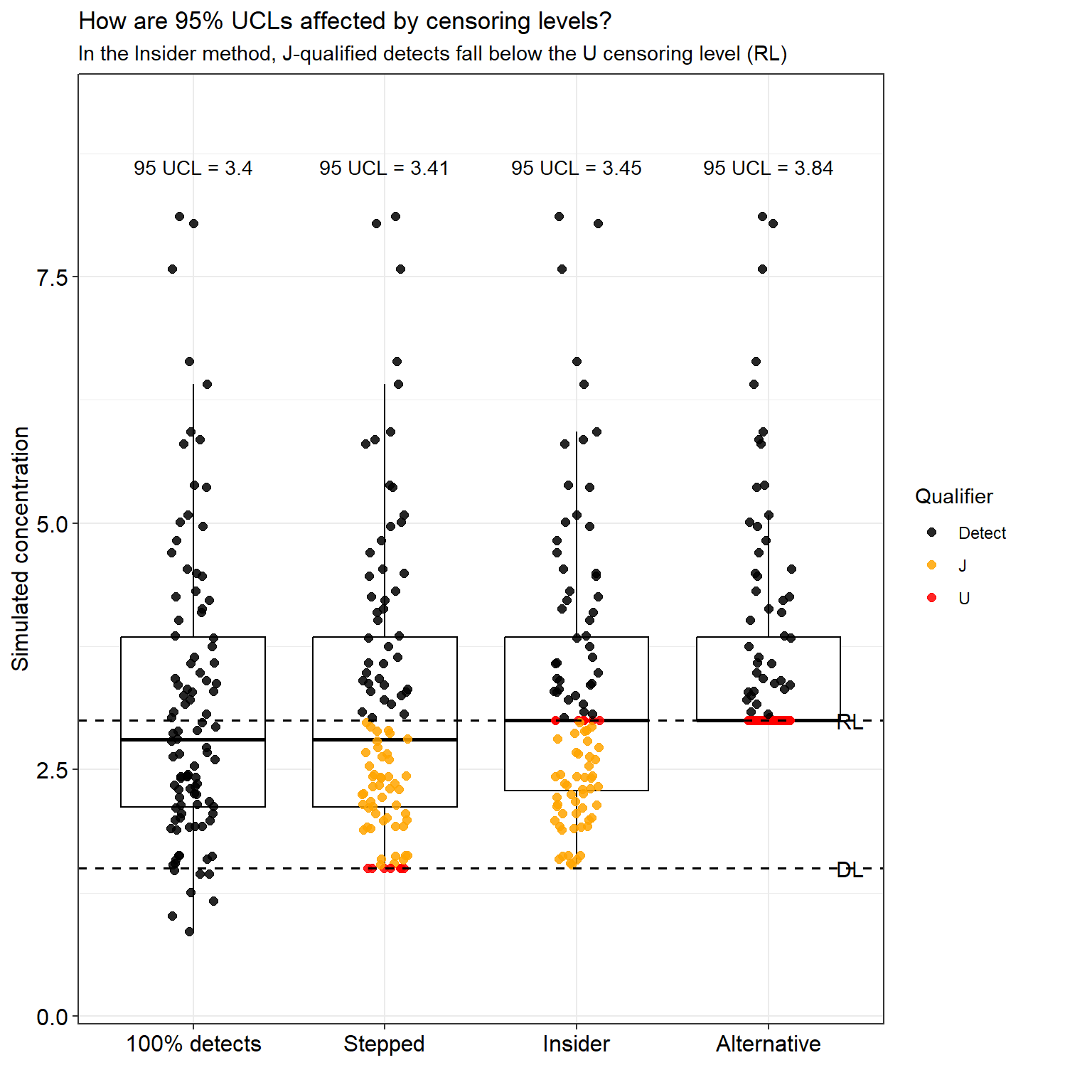
When insider censoring is applied—where nondetects are censored at the RL while J-qualified detects remain below it—the estimated 95% UCL increases relative to approaches that treat censoring more consistently, demonstrating how this practice can bias statistical results. Under the alternative approach, both U-qualified nondetects and J-qualified values below the RL are assigned the RL. Although this preserves internal consistency in the censoring level, this produces a higher 95% UCL than the unbiased or stepped approaches.
Results
The simulation illustrates how different reporting conventions influence statistical summaries derived from the same underlying dataset. When insider censoring is applied, the lower tail of the distribution is distorted and the estimated 95% UCL of the mean increases relative to approaches that apply consistent censoring thresholds. Probability plots further show that insider censoring introduces curvature in the lower tail, reflecting the redistribution of observations created by mixed censoring levels. In contrast, approaches that apply a consistent censoring limit preserve the expected distributional structure and produce more stable statistical estimates.
Because this bias originates during data preprocessing rather than statistical modeling, analysts should review how nondetect and J-qualified results are handled before conducting formal analyses. When mixed censoring thresholds are present, analysts should apply a consistent censoring limit or treat measurements between the detection and reporting limits as interval-censored observations. Clear documentation of these decisions is essential to ensure that statistical results remain transparent, reproducible, and appropriate for regulatory use.
Recommended Approaches
When insider censoring is present or suspected, several approaches can be used to minimize its impact on statistical analyses. One approach is to apply a consistent censoring limit across the dataset. For example, values below the DL would be censored at the DL, while values between the DL and RL would be retained as individual J-qualified results. Although this approach reduces bias introduced by inconsistent reporting thresholds, it may also discard information contained in measured values between the detection and reporting limits. Alternatively, the RL could be used as the censoring limit. Under this approach, all values below the RL are reported as censored. This is more conservative and discards some information, but it avoids the mixed-threshold bias created by insider censoring.
A more statistically rigorous approach is to treat observations between the DL and RL as interval-censored data. In this framework, concentrations known to fall within a specific range are treated as intervals rather than exact values. Statistical methods designed for censored data can then be applied to estimate summary statistics and distributional parameters without introducing systematic bias (Helsel, 2005; Helsel, 2012).
In general, interval-censored analysis provides the most statistically rigorous treatment because it preserves the information contained in J-qualified results. When this approach is not feasible, analysts should apply a single consistent censoring threshold. Mixed censoring thresholds should be avoided because they introduce structural bias.
Regardless of the approach used, how detection limits and reporting limits are handled during data preparation and analysis should be documented. Transparent documentation helps ensure that statistical results are reproducible and that the implications of censoring decisions are clearly understood.
Conclusions
Insider censoring occurs when nondetect results are censored at the RL while detected measurements are still reported below that threshold. This situation commonly arises when nondetect values are replaced with the RL during preprocessing, while J-qualified detections between the DL and RL are retained. This practice violates a key assumption underlying censored-data methods—that the censoring process remain noninformative with respect to the underlying concentrations.
By introducing insider censoring, the relationship between the observed measurements and the censoring mechanism is altered. As a result, the data no longer support unbiased percentile estimates, and the resulting bias propagates into common summaries and hypothesis tests. The simulation presented here illustrates these effects: the apparent distribution shifts upward, the lower tail becomes distorted, and estimated statistics differ from those obtained using more consistent analytical approaches. Consequently, the same underlying data may lead to different regulatory conclusions depending solely on preprocessing choices.
Detection limits are an inherent feature of analytical chemistry, and the primary concern is not their existence but how measurements near those limits are reported and incorporated into statistical analyses. When reporting conventions fail to clearly distinguish between true nondetections and measurable but uncertain values, structural bias can be introduced into the dataset. Careful reporting and appropriate statistical treatment of censored observations are therefore necessary to ensure that environmental datasets accurately represent the underlying measurements and support reliable scientific conclusions.
More broadly, these results highlight how seemingly routine data preprocessing decisions can materially influence statistical inference and environmental decision-making, underscoring the importance of transparent and statistically consistent handling of measurements reported near detection limits.
References
Helsel, D.R. 2005. Insider Censoring: Distortion of Data with Nondetects. Human and Ecological Risk Assessment 11, 1127-1137.
Helsel, D.R. 2012. Statistics for Censored Environmental Data Using Minitab and R, 2nd Edition. John Wiley & Sons
Millard, S.P. EnvStats: An R Package for Environmental Statistics. Springer.
R Core Team. 2026. R: A Language and Environment for Statistical Computing. R Foundation for Statistical Computing, Vienna, Austria. https://www.R-project.org.
- Posted on:
- March 15, 2026
- Length:
- 16 minute read, 3259 words
- See Also: