Introduction

Simple linear regression (regression with a single explanatory variable), and multiple linear regression (regression with multiple explanatory variables), correspond to very different questions. The former uses regression to describe univariate associations between a dependent variable and a (single) independent variable. Simple regression is a measure of the direct effect of a single explanatory variable on the response variable under the assumption that there are no strong indirect influences through any additional third variables. These interpretations require that a linear function provides a reasonable model of the relationship between the explanatory variable and the response variable. Multiple regression simultaneously describes the direct effects of multiple explanatory variables on a response, accounting for the direct effects of each explanatory variables included in the model. These estimated direct effects are called partial regression coefficients. Partial regression coefficients represent how much the response variable would increase, per unit increase of a given explanatory variable, if the value of the explanatory variable was increased while holding the values of all other explanatory variables constant.

Univariate regression models are the simplest model, by definition. However, most environmental phenomena are not simple but depend on multiple variables, and in a complex manner. A linear regression model based on one variable at a time will most likely have a high bias. Although simple regression models may help identify the most essential feature in a dataset, multivariant analyses are required to fully understand correlation patterns and leverage the data for accurate decision making. Multiple regression allows the interpretation of regression coefficients in terms of the other explanatory variables. For example, simple regression allows one to determine the effect that x has on y and the effect that z has on y. If x and z are related statistically, then simply regressing y on x will give an erroneous estimate of the effect of x on y because some of the effect of z will be incorporated in the regression. The same thing happens when regressing y on z. Even if x and z are perfectly orthogonal, accounting for the variance explained by z when looking at the relationship between x and y can reduce variation, resulting in a more precise model.

Having a large number of variables invites additional issues in using classic regression models. One alternative to ordinary least squares regression is to use regularized regression (also commonly referred to as penalized models or shrinkage methods) to constrain the total size of all the coefficient estimates (Hastie et al. 2016; Kuhn and Johnson 2016). Regularization is a technique that prevents the parameters of a model from becoming too large and “shrinks” them toward zero. Three particularly well-known and commonly used regularization techniques for linear models are:

• Ridge regression
• Least absolute shrinkage and selection operator (LASSO)
• Elastic net

These three techniques can be thought of as extensions to original least squares regression. Because they shrink model parameters toward zero, they can also automatically perform variable selection by forcing explanatory variables with little information to have no or negligible impact on predictions.

Ridge Regression

The principal job of regularization is to discourage model complexity by penalizing model parameters that are large, shrinking them toward zero. Ridge regression modifies the least squares loss function slightly to include a term that increases the function’s value for larger parameter estimates. As a result, the algorithm now has to balance selecting the model parameters that minimize the sum of squares, and selecting parameters than minimize this new penalty. Recall that original least squares regression minimizes the sum of the squared errors (SSE):

$$SSE = \sum_{i=1}^{n}(y_i - \hat{y_i})^2$$

In ridge regression, this penalty is called the L2 norm, and is given by the sum of the squared regression parameters (except the intercept) (Hoerl 1970):

$$SSE_{L2} = \sum_{i=1}^{n}(y_i - \hat{y_i})^2 + \lambda\sum_{j=1}^{P}\beta_j^2$$

where \(\lambda\ge 0\) is a tuning parameter, to be determined separately. When \(\lambda = 0\), the penalty term has no effect, and ridge regression will produce the least squares estimates. However, as \(\lambda \to \infty\), the impact of the shrinkage penalty increases, and the ridge regression coefficient estimates will approach zero. The “L2” signifies that a second-order penalty (i.e., the square) is being used on the parameter estimates. The effect of this penalty is that the parameter estimates are only allowed to become large if there is a proportional reduction in SSE. In effect, this method shrinks the estimates towards zero as the \(\lambda\) penalty becomes large. Although some parameter estimates become negligibly small, ridge regression does not shrink values to absolute zero for any value of the penalty.

LASSO

An alternative to ridge regression is the LASSO method (Tibshirani 1996), which uses the L1 norm to shrink parameter estimates. The L1 norm is only slightly different than the L2 norm. Instead of squaring the regression parameter values, LASSO uses the sum of their absolute value:

$$SSE_{L1} = \sum_{i=1}^{n}(y_i - \hat{y_i})^2 + \lambda\sum_{j=1}^{P}\vert{\beta_j}\vert$$

The “L1” signifies that a first-order penalty is being used on the parameter estimates. In the case of the LASSO, the L1 penalty has the effect of forcing some of the coefficient estimates to be exactly equal to zero when the tuning parameter \(\lambda\) is sufficiently large. Thus, the LASSO simultaneously uses regularization to improve model performance and to conduct variable selection.

Elastic Net

Elastic net combines both the L1 and L2 norms to find a compromise between ridge regression and LASSO parameter estimate (Zou and Hastie 2005):

$$SSE_{Enet} = \sum_{i=1}^{n}(y_i - \hat{y_i})^2 + \lambda\left((1 - \alpha)\sum_{j=1}^{P}\beta_j^2 + \alpha\sum_{j=1}^{P}\vert{\beta_j}\vert\right)$$

The “Enet” signifies that a combination of first-order and second-order penalties is being used on the parameter estimates. The advantage of this model is that it enables effective regularization via the ridge-type penalty with the feature selection quality of the LASSO. Both the penalties require tuning to achieve optimal performance. This can be accomplished using cross-validation. The \(\alpha\) parameter can take any value between 0 and 1:

• When \(\alpha = 0\), the L1 norm becomes 0 (pure ridge regression).
• When \(\alpha = 1\), the L2 norm becomes 0 (pure LASSO).
• When \(0 < \alpha < 1\), there is a mixture of ridge regression and LASSO.

Centering and Scaling

The key statistic of linear regression is the slope of the fitted linear function. Interpreting the slope is useful because it predicts how the outcome variable changes with the explanatory variables. Centering variables doesn’t affect the slopes in non-penalized linear regression because the relationships between variables remain the same. Therefore, predictions made using linear regression are unaffected by centering and scaling of the data. When using L1- or L2-penalized loss functions, it’s critical that the explanatory variables are scaled first (divided by their standard deviation) to remove the influence of different input variable units. Because the squared slopes (in the case of L2 regularization) are being used in the loss function, the penalty is going to be considerably larger for explanatory variables on larger scales. If explanatory variables are not scaled first, they won’t all be given equal importance.

Example

Let’s compare results from simple linear regression and multiple linear regression with and without shrinkage. For this example, let’s use a dataset consisting of indoor air concentrations of trichloroethene (TCE) and various explanatory variables, including radon concentration, temperature, barometric pressure, wind direction, and wind speed.

Data

Data quality is an important issue for any project analyzing data. Prior to conducting any statistical analyses, it’s important to analyze the data using various statistical and visualization techniques to bring important aspects of the data into focus for further analysis. Specifically, it’s important to get an understanding of:

• The properties of the data, such as schema and statistical properties;
• The quality of the data, like missing values, outliers, and inconsistent data types; and
• The predictive power of the data, such as correlation of features against the target variable.

For brevity, let’s assume that we have performed a thorough explanation of the data. The data consist of 11 variables with 1,193 observations averaged over 6-hour internals. The variables include the following:

• Barometric pressure, atmosphere (BP)
• Date, m/d/yyyy
• Differential temperature (DT)
• Differential pressure (DP)
• Outside temperature, Fahrenheit (Temp)
• Precipitation, inches of water (Precip)
• Radon concentration, picocuries per liter (Radon)
• TCE concentration, micrograms per cubic meter (TCE)
• Wind speed, miles per hour (WindSpeed)
• Wind direction (WindDir)
• Working hour, defined as 6am to 6pm Monday through Friday (WorkHr)

Let’s look at the structure of the data.

# Load libraries
library(tidyverse)
library(recipes)
library(mlr)

# Load the data
dat <- read.csv('./data/NESDI_EIA11data_MVA_20200402.csv', header = T,
                na.strings = c("", "NA"),
                stringsAsFactors = FALSE)
dat$Date <- as.POSIXct(dat$Date, format = '%m/%d/%Y %H:%M', tz = 'EST')

# Change BP from integer to numeric
dat$BP <- as.numeric(dat$BP)

# Convert temperature from Celsius to Fahrenheit
dat$Temp <- (9/5) * dat$Temp + 32

# Convert barometric pressure from Pascal to atmosphere
dat$BP <- dat$BP/101325

# View data structure
str(dat)

## 'data.frame':	1193 obs. of  11 variables:
##  $ Date     : POSIXct, format: "2019-05-17 06:00:00" "2019-05-17 12:00:00" ...
##  $ WorkHr   : chr  "Y" "Y" "N" "N" ...
##  $ Temp     : num  72.5 83.6 75 67.9 74.7 ...
##  $ WindSpeed: num  9.97 12.84 3.64 7.04 3.07 ...
##  $ WindDir  : chr  "SSW" "SW" NA "SSW" ...
##  $ BP       : num  1 0.997 0.998 1 1.003 ...
##  $ Precip   : num  0 0 0 0.17 0 0 0 0 0 0 ...
##  $ Radon    : num  0.68 0.27 0.23 0.36 0.48 0.3 0.27 0.34 0.29 0.39 ...
##  $ DP       : num  0.004 0.003 0.006 0.003 0.005 0.004 0.005 0.007 0.007 0.005 ...
##  $ DT       : num  0.08 -5.97 -1.28 2.68 -1.12 -2.01 1.01 1.82 -3.63 -9.9 ...
##  $ TCE      : num  0.77 0.22 0.3 0.45 0.36 0.37 0.43 0.5 0.41 0.4 ...

Prior to conducting the regresssion, missing values for the explanatory variables were imputed using bagged decision trees. Bagging is the application of the bootstrap procedure (random sampling with replacement) applied to decision trees. Wind direction was converted to an ordered factor with missing values assigned “ND” for “no direction”. Numeric conversion of wind direction was achieved using label encoding (also referred to as ordinal encoding). One-hot encoding was used to generate a full-rank encoding of working hour. Log transformation was applied to the response variable TCE to stabilize non-constant variance. Additionally, differential temperature was removed from the dataset because it was shown to be highly correlated with outside temperature. The lag-1 value for TCE was included as an explanatory variable to account for the presence of serial correlation.

# Assign "ND" to missing wind direction values
dat <- dat %>%
   mutate(WindDir = replace(WindDir, is.na(WindDir), "ND"))

# Create wind direction levels
wind_lvls <- c("N", "NNE", "NE", "ENE", "E",
               "ESE", "SE", "SSE", "S", "SSW",
               "SW", "WSW", "W", "WNW", "NW",
               "NNW", "ND")

# Create ordered factor
dat$WindDir <- factor(dat$WindDir, levels = wind_lvls,
                      ordered = TRUE)

# Remove Data with Missing TCE
dat2 <- subset(dat, !is.na(TCE))

# Remove DT because it is highly correlated with temp
dat2$DT <- NULL

# Replace Replace BP anomaly with mean of values before and after
rn <- which.min(dat2$BP)
newBP <- mean(dat2[(rn - 1), "BP"][[1]], 
              dat2[(rn + 1), "BP"][[1]])
newDP <- mean(dat2[(rn - 1), "DP"][[1]], 
              dat2[(rn + 1), "DP"][[1]])
dat2[rn, "BP"] <- newBP
dat2[rn, "DP"] <- newDP

# Log transformation of TCE
dat2$TCE <- log10(dat2$TCE)

# Impute using bagged trees
rec <- recipe(TCE ~ ., data = dat2[ -1])
impute_rec <- rec %>%
  step_bagimpute(all_predictors()) %>%
  step_ordinalscore(WindDir) %>%
  step_dummy(WorkHr, one_hot = FALSE) %>%
  step_lag(TCE, lag = 1) %>%
  step_naomit(all_predictors())

imp_models <- prep(impute_rec, training = dat2)
dat2_imputed <- bake(imp_models, new_data = dat2, everything())

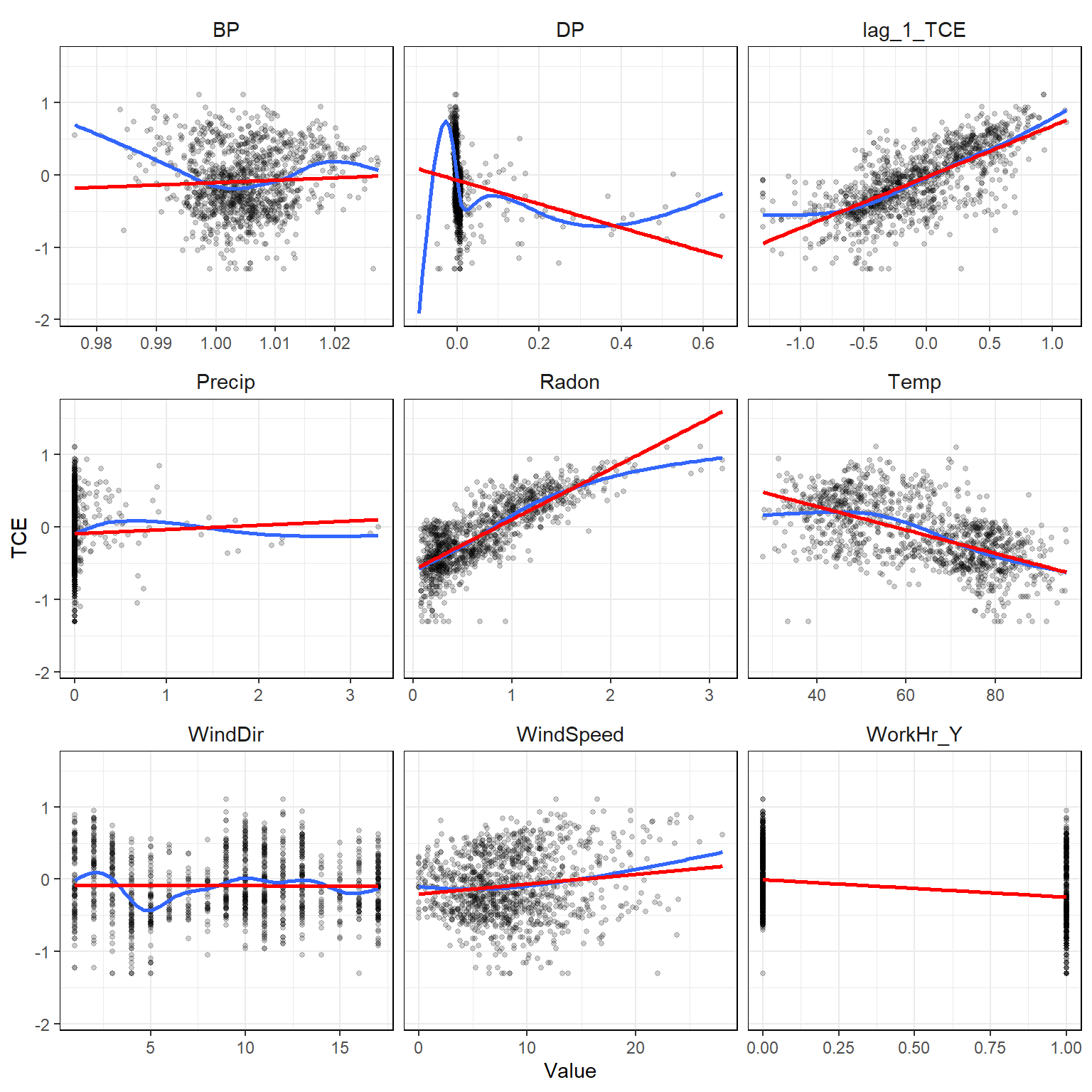
Let’s plot the data to get a better understanding of the relationships within it. In the resulting plots, the red lines represent simple linear model fits between each explanatory variable and TCE. The blue line represents a generalized additive model. It appears that Radon strongly correlates with TCE, although, the relationship appears to be nonlinear.

# Plot the data
# Format data for plotting
dat2_imputed_long <- dat2_imputed %>%
  gather(key = "Variable", value = "Value", -TCE)

# Create x-y plots
ggplot(data = dat2_imputed_long, aes(x = Value, y = TCE)) +
  geom_point(size = 1, alpha = 0.2) +
  geom_smooth(method = "gam", se = FALSE) +
  geom_smooth(method = "lm", formula = "y ~ x", se = FALSE, col = "red") +
  facet_wrap(~ Variable, ncol = 3, scale = "free_x") +
  theme_bw() +
  theme(strip.text = element_text(size = 11),
        strip.background = element_rect(color = NA, fill = NA),
        panel.border = element_rect(fill = NA, color = "black"))

Simple Linear Regression

Let’s regress TCE on each of the explanatory variables and inspect the regression coefficients.

mod_list <- dat2_imputed %>% 
  as_tibble %>% 
  gather(key = "Variable", value = "Value", -TCE) %>%
  nest(data = c(TCE, Value)) %>%
  mutate(model = map(data, ~lm(TCE ~ Value, data = .))) %>%
  mutate(tidy_model = map(model, tidy)) %>%
  select(-data, -model) %>%
  unnest(cols = c(tidy_model))     

# Create all models
mod_list <- dat2_imputed %>% 
  as_tibble %>% 
  gather(key = "Variable", value = "Value", -TCE) %>%
  nest(data = c(TCE, Value)) %>%
  mutate(model = map(data, ~lm(TCE ~ Value, data = .))) %>%
  mutate(tidy_model = map(model, tidy))

# Get coefficients
lmSingleCoefs <- mod_list %>%
  select(-data, -model) %>%
  unnest(cols = c(tidy_model)) %>%
  filter(term != '(Intercept)') %>%
  select(-term)
lmSingleCoefs

## # A tibble: 9 x 5
##   Variable   estimate std.error statistic   p.value
##   <chr>         <dbl>     <dbl>     <dbl>     <dbl>
## 1 Temp      -0.0163    0.000699  -23.3    6.07e- 98
## 2 WindSpeed  0.0137    0.00285     4.80   1.78e-  6
## 3 WindDir   -0.000245  0.00268    -0.0912 9.27e-  1
## 4 BP         3.28      1.90        1.72   8.50e-  2
## 5 Precip     0.0588    0.0581      1.01   3.11e-  1
## 6 Radon      0.699     0.0158     44.2    2.34e-246
## 7 DP        -1.64      0.243      -6.76   2.25e- 11
## 8 WorkHr_Y  -0.241     0.0276     -8.75   7.83e- 18
## 9 lag_1_TCE  0.705     0.0214     33.0    1.93e-166

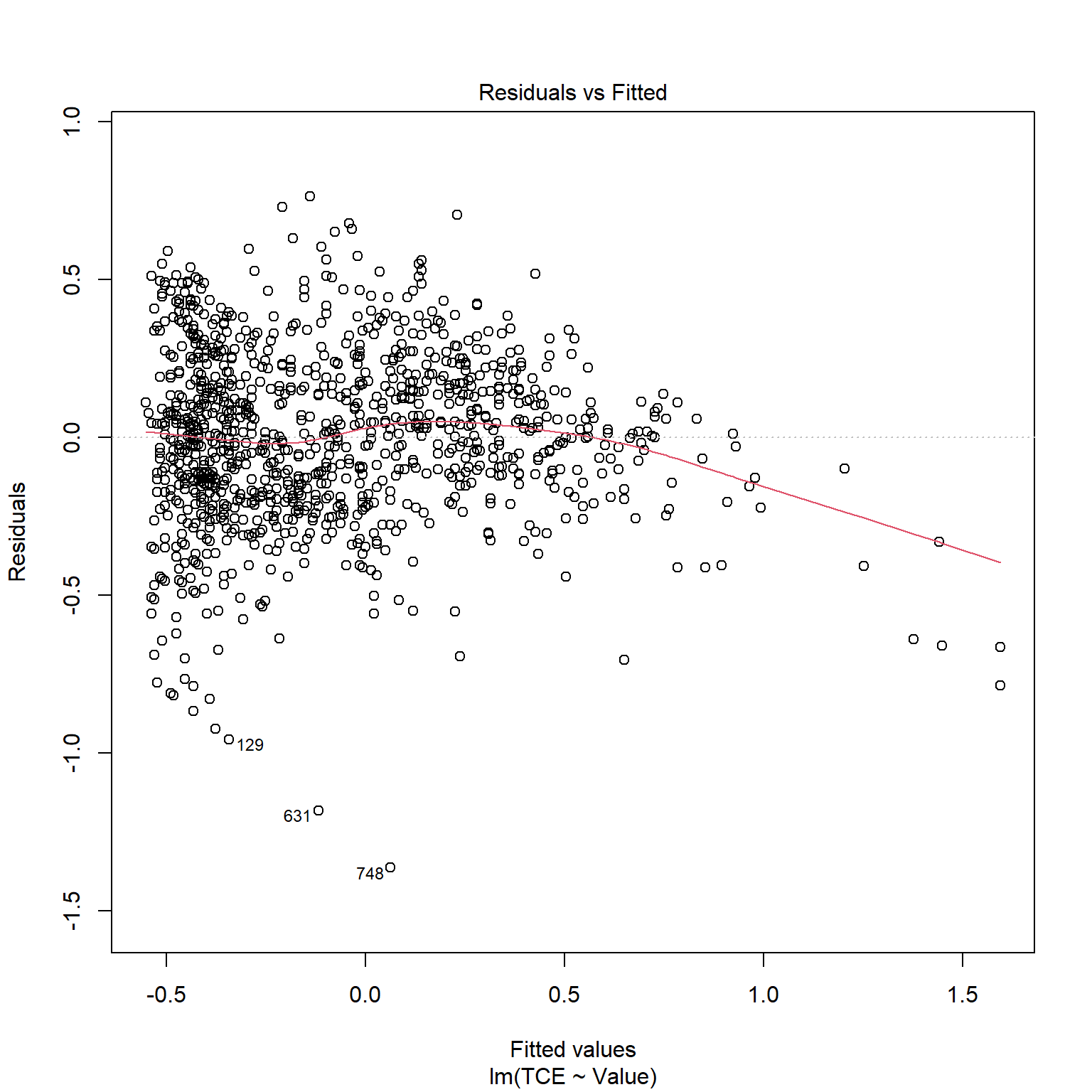
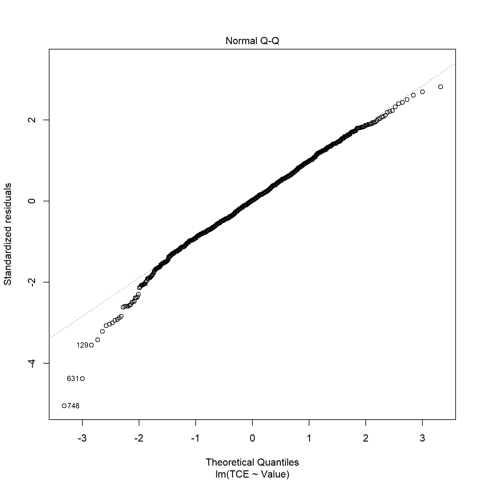
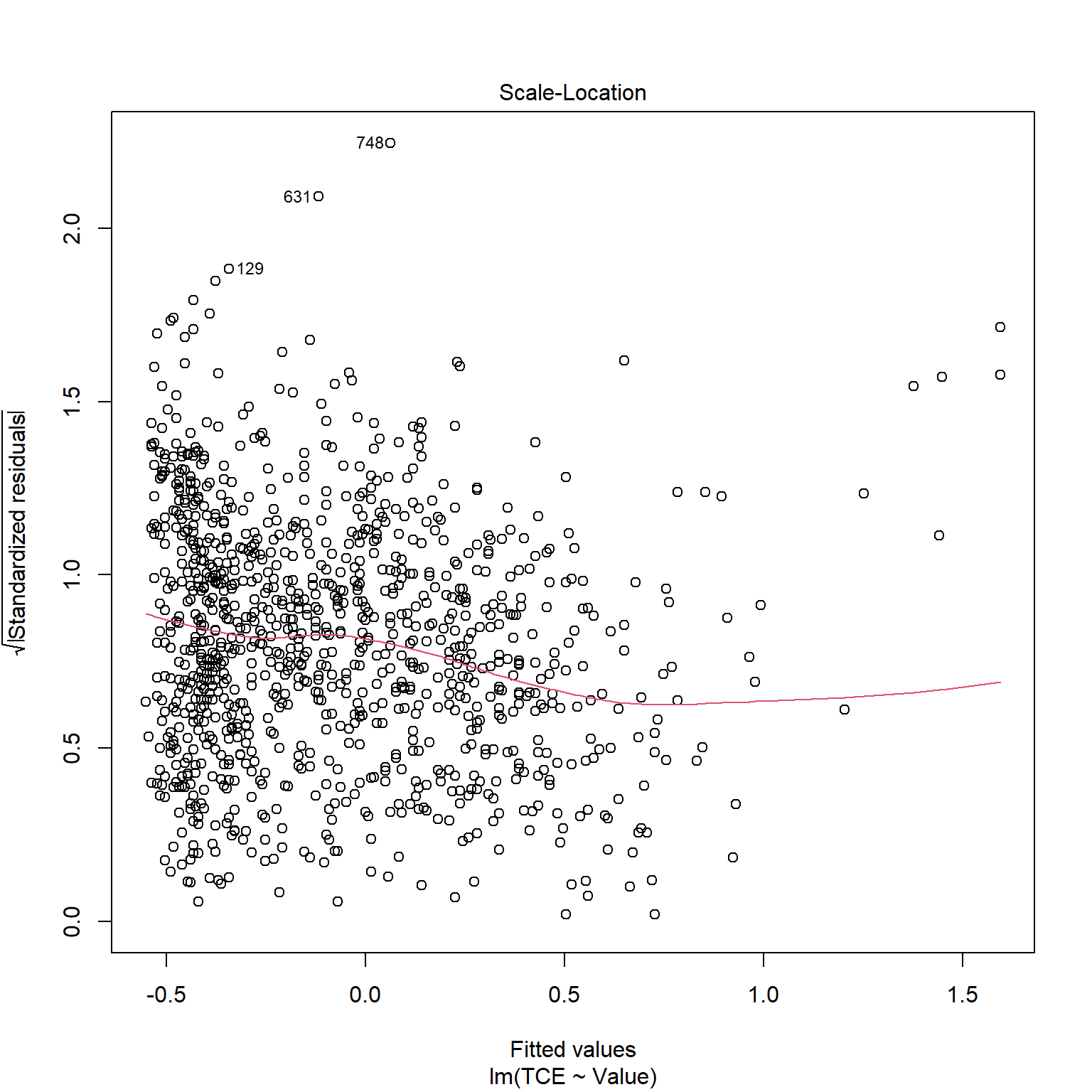
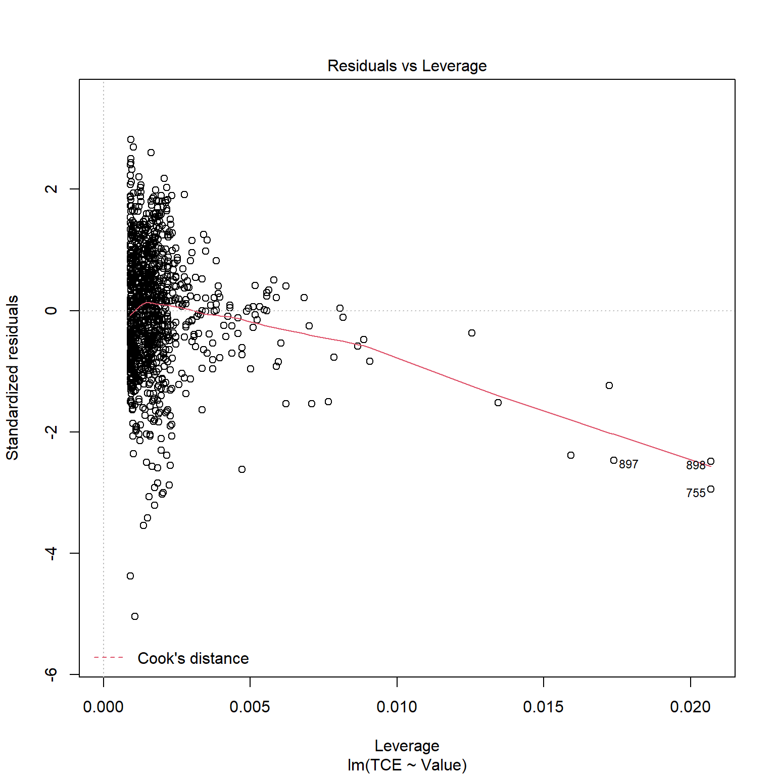
TCE appears to be strongly correlated to Radon levels. Let’s quickly inspect the diagnotics plots to assess whether a linear model is appropriate. When a linear model is appropriate, we expect the residuals will have constant variance when plotted against fitted values and the residuals and fitted values will be uncorrelated. There are clear indicators in the residual plot that the given linear model is inappropriate.

# Inspect model diagnostics
plot(mod_list$model[[6]])

Multiple Linear Regression

Let’s perform multiple linear regression for comparison with simple linear regression and penalized regression. Recall how important it is to scale the explanatory variables when calculating the L1 and/or L2 norms. Let’s use the same process here for consistency so we can easily compare the results to those obtained using penalized regression. After performing the regression, we will transform the parameters back into their original scale for reporting.

# Make lm task and learner
tceTask <- makeRegrTask(data = dat2_imputed, target = "TCE")
lin <- makeLearner("regr.glmnet", alpha = 0, id = "lm")

# Train model
lmM <- setHyperPars(lin, par.vals = list(s = 0))  # set lambda to 0
lmModel <- train(lmM, tceTask)

# Get model data
lmModelData <- getLearnerModel(lmModel)
lmCoefs <- coef(lmModelData, s = 0)
lmCoefs

## 10 x 1 sparse Matrix of class "dgCMatrix"
##                       s1
## (Intercept)  0.370624464
## Temp        -0.002279429
## WindSpeed    0.001106128
## WindDir     -0.001472800
## BP          -0.493146632
## Precip       0.057469950
## Radon        0.389939199
## DP          -0.201658580
## WorkHr_Y    -0.192715127
## lag_1_TCE    0.355751157

Ridge Regression

Let’s train a ridge regression model to predict TCE from our dataset. We will tune \(\lambda\) and train the model using its optimal value. Let’s define our search method for \(\lambda\) as a random search between 0 and 1 using 200 iterations and 3-fold cross-validation repeated 5 times. Similar to the multiple regression model, we will scale the explanatory variables for the penalized regression and back transform the parameters into their original scale for reporting. We will apply this same process to the LASSO and elastic net regression models.

# Load libraries
library(parallel)
library(parallelMap)
library(RColorBrewer)

# Make ridge task and learner
ridge <- makeLearner("regr.glmnet", alpha = 0, id = "ridge")

# Tuning the lambda (s) hyperparameter
set.seed(52134)
ridgeParamSpace <- makeParamSet(
  makeNumericParam("s", lower = 0, upper = 1))
randSearch <- makeTuneControlRandom(maxit = 200)
cvForTuning <- makeResampleDesc("RepCV", folds = 3, reps = 10)

parallelStartSocket(cpus = detectCores())
tunedRidgePars <- tuneParams(ridge, task = tceTask,
                            resampling = cvForTuning, 
                            par.set = ridgeParamSpace, 
                            control = randSearch)
parallelStop()
tunedRidgePars

## Tune result:
## Op. pars: s=0.0123
## mse.test.mean=0.0533952

# Train a ridge regression model using the tuned lambda
tunedRidge <- setHyperPars(ridge, par.vals = tunedRidgePars$x)
tunedRidgeModel <- train(tunedRidge, tceTask)

# Extract the model parameters
ridgeModelData <- getLearnerModel(tunedRidgeModel)
ridgeCoefs <- coef(ridgeModelData, s = tunedRidgePars$x$s)
ridgeCoefs

## 10 x 1 sparse Matrix of class "dgCMatrix"
##                       s1
## (Intercept)  0.370624464
## Temp        -0.002279429
## WindSpeed    0.001106128
## WindDir     -0.001472800
## BP          -0.493146632
## Precip       0.057469950
## Radon        0.389939199
## DP          -0.201658580
## WorkHr_Y    -0.192715127
## lag_1_TCE    0.355751157

# Get model parameters for plotting
coefTib <- tibble(Coef = rownames(ridgeCoefs)[-1],
                  Ridge = as.vector(ridgeCoefs)[-1],
                  Lm = as.vector(lmCoefs)[-1],
                  Lm_Simple = as.vector(lmSingleCoefs$estimate))
coefLong <- gather(coefTib, key = Model, value = Beta, -Coef)

LASSO

Let’s train a LASSO model to predict TCE from our dataset. Similar to ridge regression, we will tune \(\lambda\) and train the model using its optimal value. Let’s define our search method for \(\lambda\) as a random search between 0 and 1 using 200 iterations and 3-fold cross-validation repeated 5 times.

# Make LASSO Learner
lasso <- makeLearner("regr.glmnet", alpha = 1, id = "lasso")

# Tuning lamba for LASSO
set.seed(52134)
lassoParamSpace <- makeParamSet(
  makeNumericParam("s", lower = 0, upper = 1))
randSearch <- makeTuneControlRandom(maxit = 200)
parallelStartSocket(cpus = detectCores())
tunedLassoPars <- tuneParams(lasso, task = tceTask,
                             resampling = cvForTuning, 
                             par.set = lassoParamSpace, 
                             control = randSearch)
parallelStop()
tunedLassoPars

## Tune result:
## Op. pars: s=0.0116
## mse.test.mean=0.0531059

# Train a LASSO model using the tuned lambda
tunedLasso <- setHyperPars(lasso, par.vals = tunedLassoPars$x)
tunedLassoModel <- train(tunedLasso, tceTask)

# Extract model parameters
lassoModelData <- getLearnerModel(tunedLassoModel)
lassoCoefs <- coef(lassoModelData, s = tunedLassoPars$x$s)
lassoCoefs

## 10 x 1 sparse Matrix of class "dgCMatrix"
##                        s1
## (Intercept) -0.2488541632
## Temp        -0.0009198233
## WindSpeed    .           
## WindDir      .           
## BP           .           
## Precip       0.0134860476
## Radon        0.4315498400
## DP           .           
## WorkHr_Y    -0.1800807321
## lag_1_TCE    0.3576158313

# Get model parameters for plotting
coefTib$LASSO <- as.vector(lassoCoefs)[-1]
coefLong <- gather(coefTib, key = Model, value = Beta, -Coef)

Elastic Net Regression

Let’s train an elastic net model to predict TCE from our dataset. We will tune both \(\lambda\) and \(\alpha\) and use the optimal values to train the model. Let’s define our search method for \(\lambda\) and \(\alpha\) as a random search between 0 and 1 using 400 iterations and 3-fold cross-validation repeated 5 times. Bcause we are tuning two hyperparameters simultaneously, we increased the number of iterations of our random search to get a little more coverage of the search space.

# Make elastic net Learner
elastic <- makeLearner("regr.glmnet", id = "elastic")

# Tune lambda and alpha for elastic net
set.seed(52134)
elasticParamSpace <- makeParamSet(
  makeNumericParam("s", lower = 0, upper = 1),
  makeNumericParam("alpha", lower = 0, upper = 1))

randSearchElastic <- makeTuneControlRandom(maxit = 400)
parallelStartSocket(cpus = detectCores())
tunedElasticPars <- tuneParams(elastic, task = tceTask,
                             resampling = cvForTuning, 
                             par.set = elasticParamSpace, 
                             control = randSearchElastic)
parallelStop()
tunedElasticPars

## Tune result:
## Op. pars: s=0.0134; alpha=0.312
## mse.test.mean=0.0529949

# Train an elastic net model using tuned hyperparameters
tunedElastic <- setHyperPars(elastic, par.vals = tunedElasticPars$x)
tunedElasticModel <- train(tunedElastic, tceTask)

# Extract model parameters
elasticModelData <- getLearnerModel(tunedElasticModel)
elasticCoefs <- coef(elasticModelData, s = tunedElasticPars$x$s)
elasticCoefs

## 10 x 1 sparse Matrix of class "dgCMatrix"
##                        s1
## (Intercept) -1.988605e-01
## Temp        -1.411240e-03
## WindSpeed    5.749234e-05
## WindDir     -6.656216e-04
## BP           .           
## Precip       4.473929e-02
## Radon        4.193089e-01
## DP          -1.095286e-01
## WorkHr_Y    -1.924013e-01
## lag_1_TCE    3.654960e-01

# Get model parameters for plotting
coefTib$Elastic <- as.vector(elasticCoefs)[-1]
coefLong <- gather(coefTib, key = Model, value = Beta, -Coef)

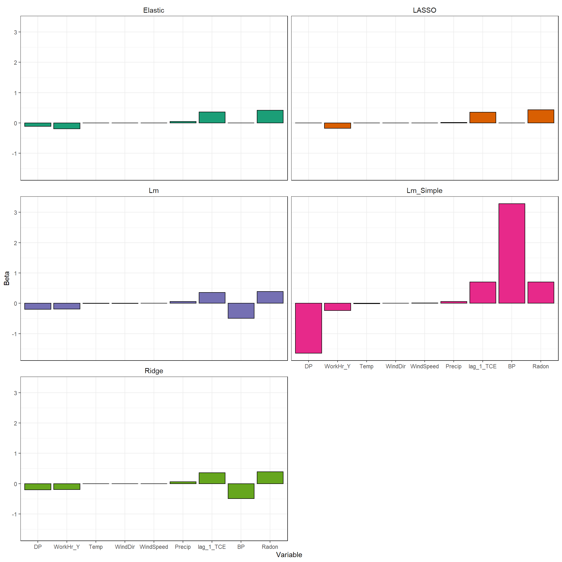
Now that we have trained all the models, let’s plot the parameter estimates to see the effect of parameter shrinkage. For the LASSO, 4 of the 10 variables have been removed from the model completely - the slopes of these parameters have been set to exactly zero. These variables include BP, DP, WindDr, and WindSpeed. This is how LASSO can be used for performing feature selection. The elastic net parameter estimates are similar to those of the LASSO, with 3 of the 10 variables removed from the model. DP was retained in the elastic net model but was removed from the LASSO. Radon, lag_1_TCE. and WorkHr_Y have the highest parameter estimates in both the elastic net and LASSO models.

# Plot the model parameters
ggplot(coefLong, aes(reorder(Coef, Beta), Beta, fill = Model)) +
  geom_bar(stat = "identity", position = "dodge", col = "black") +
  facet_wrap(~ Model, ncol = 2) +
  labs(x = 'Variable') +
  scale_fill_brewer(palette = "Dark2") +
  theme_bw() +
  theme(legend.position = "none") +
  theme(strip.text = element_text(size = 11),
        strip.background = element_rect(color = NA, fill = NA),
        panel.border = element_rect(fill = NA, color = "black"))

Model Residuals

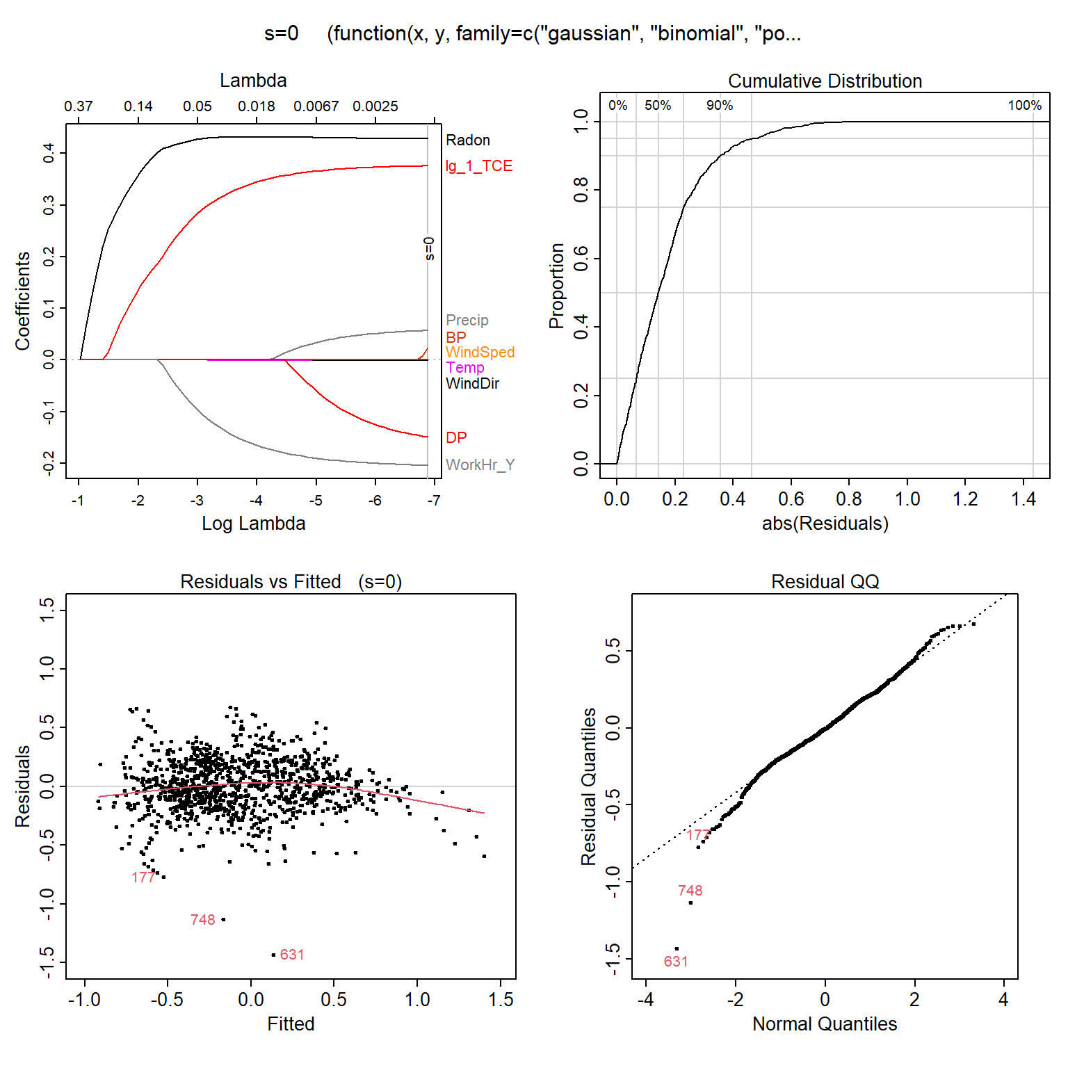
The assumptions and conditions for multiple regression model are nearly the same as for simple regression. They assume that residuals are normally distributed and homoscedastic (constant variance). Let’s quickly inspect the diagnotics plots for the LASSO to assess whether these assumptions are valid. The Residuals vs. Fitted plot shows the predicted TCE concentration on the x-axis and the residual on the y-axis for each case. We hope that there are no patterns in this plot (the amount of error does not depend on the predicted value). In this situation, we have a curved relationship, indicating nonlinear relationships between explanatory variables and TCE, and/or non-constant variance.

# Load libraries
library(plotmo)

# Plot residuals of LASSO regression model
plotres(lassoModelData)

Conclusion

In general, the LASSO performs better when there are a few explanatory variables that have large coefficients, and the remaining variables have coefficients that are very small or equal to zero. Ridge regression performs better when the response is a function of many explanatory variables, all with coefficients of roughly equal size (James et al. 2017). In situations where the relationship between the response and the explanatory variables is close to linear, the least squares estimates will have low bias but may have high variance. This means that a small change in the data can cause a large change in the least squares coefficient estimates. In particular, when the number of variables p is almost as large as the number of observations n, the least squares estimates will be extremely variable. If p > n, least squares will not have a unique solution, whereas ridge regression can still perform well. As with ridge regression, when the least squares estimates have excessively high variance, the LASSO can yield a reduction in variance at the expense of a small increase in bias, and consequently can generate more accurate predictions. Unlike ridge regression, the LASSO provides models that are easier to interpret via its variable selection.

When modeling data with a linear model, we make the assumption that our residuals are normally distributed and homoscedastic. For models built to explain, it is important to check model assumptions, such as the distribution of residuals. Irregularities in the data or misspecifications of the relationships between the explanatory variables and the response variable can result in a highly inaccurate model. For instance, you may conclude that a predictor and a response variable are unrelated when, in fact, they are. Alternatively, you may conclude that a predictor and a response variable are related when, in fact, they are not.

Linear regression can have significant limitations because the linearity assumption is almost always an approximation. As evident in this example, the relationship between the explanatory variables and TCE appears to be nonlinear. A better modelling choice may be random forest regression. Random forests have become a popular and widely-used tool for nonparametric regression in many scientific areas. They show high predictive accuracy and are applicable even in high-dimensional problems with highly correlated variables.

References

Hastie, T., R. Tibshirani, and J. Friedman. 2016. The Elements of Statistical Learning: Data Mining, Inference, and Prediction, Second Edition. Springer, New York.

Hoerl, A. E and R. W Kennard. 1970. Ridge regression: Biased estimation for nonorthogonal problems. Technometrics 12, 55-67.

James, G., D. Witten, T. Hastie, and R Tibshirani. 2017. An Introudction to Statistical Learning. Springer, New York.

Kuhn, M. and K. Johnson. 2016. Applied Predictive Modeling. Springer, New York.

Tibshirani, R. 1996. Regression shrinkage and selection via the lasso. J. Royal Stat. Soc.B), 73, 273-282.

Zou, H. and T. Hastie. 2005. Regularization and variable selection via the elastic net. J. Royal Stat. Soc.B, 67, 301-320.