Introduction

Segmented regression provides a practical and defensible framework for improving remediation timeframe estimates by explicitly accounting for changes in concentration trends over time. Traditional linear regression assumes a single, constant rate of decline, which can oversimplify plume behavior and lead to over- or under-estimation of cleanup duration when site conditions evolve. In contrast, segmented regression identifies statistically meaningful breakpoints in monitoring data and fits separate linear trends to each phase of plume response?such as initial rapid mass removal, transition periods, and asymptotic tailing. By quantifying distinct attenuation rates before and after these inflection points, the method better reflects underlying hydrogeologic controls, source depletion dynamics, and remedy performance. This results in more realistic projections of when concentrations are expected to achieve remedial goals, while also providing a transparent, data-driven basis for communicating uncertainty and performance expectations to regulators and stakeholders.

Background

To estimate the time required to acheive the cleanup goal, an attenuation rate was calculated for vinyl chloride at groundwater monitoring well MW-1. This estimated rate incorporates the combined effects of natural attenuation processes influencing groundwater concentrations, including advection, dispersion, sorption, transformation, volatilization, and chemical or biological degradation, as well as site-specific hydrogeologic conditions and changes in those conditions (USEPA 2004). At this site, the calculated rate also reflects the influence of ongoing groundwater treatment processes. Consistent with United States Environmental Protection Agency (USEPA) guidance and widespread field observations, groundwater contaminant concentrations typically decline in an exponential manner over time, such that a plot of the natural logarithm of concentration versus time produces a linear relationship, indicating first-order decay behavior (USEPA 2011).

The rate of attenuation is represented using a first-order rate equation, in which the rate of concentration reduction is proportional to the concentration present. The USEPA has evaluated different types of attenuation rates for monitored natural attenuation studies and concluded that first-order concentration-versus-time rate constants should be used to estimate how quickly remediation goals will be met at a site (Newell et al. 2006). Alternative approaches, such as zero-order decay, do not reliably capture source depletion behavior and can produce misleading timeframe projections.

The first-order rate equation is expressed mathematically as:

\begin{equation}\tag{1} C(t) = C_0 \cdot e^{kt} \end{equation}

where

\(C_0\) = initial concentration at the beginning of the time interval
\(C(t)\) = concentration at time t (year)
k = first-order attenuation rate constant (1/year)

Taking the natural logarithms (ln), the rate equation becomes:

\begin{equation}\tag{2} ln[C(t)] = kt + ln[C_0] \end{equation}

The first-order attenuation rate constant is given by the slope of a line that best fits the natural logarithms of the concentrations as a function of time for a given compound at a given monitoring location. This rate was used to forecast the future concentrations of vinyl chloride and predict when concentrations will attain the established cleanup goal \(C_{goal}\) at MW-1 using the following equation:

\begin{equation}\tag{3} t = \frac{ln(C_0/C_{goal})}{k} \end{equation}

Equation (3) provides a mathematically direct and statistically defensible means of projecting cleanup timeframes and evaluating whether attenuation is proceeding at a sufficient rate to achieve regulatory objectives (USEPA 2002; USEPA 2011).

Changepoint analysis improves estimates of remediation timeframes because it addresses a key limitation of traditional first-order evaluations—namely, the assumption that the attenuation rate remains constant over time. A changepoint is a statistically identifiable point in a time series where the underlying relationship between variables shifts, such as an abrupt change in the slope of a concentration-versus-time trend. Changepoint analysis, often implemented using piece-wise (segmented) linear regression, divides a monitoring record into distinct segments and fits a separate linear regression to each, with segments joined at statistically significant changepoints/breakpoints.

A recent study by Ferrey et al. (2024) demonstrates that, although contaminant attenuation is commonly modeled using a first-order concentration-versus-time regression, monitoring records often contain statistically significant shifts in slope (i.e., changes in rate constants). By identifying statistically significant shifts in attenuation rates, changepoint analysis isolates the most recent trend segment, which provides the most defensible basis for forecasting future concentrations. As a result, forecasts based solely on historic first-order regressions may under- or over-estimate cleanup timeframes, whereas segmented regression improves predictive accuracy by reflecting current plume behavior and evolving attenuation conditions.

Software

Calculations were performed using the R language for statistical computing and visualization, version 4.5.2 (R Core Team 2025). Several libraries and functions were used during the analysis as shown below. Changepoint analysis and segmented regression was performed using the segmented (Muggeo 2026) library. The library can be used to estimate linear and generalized linear models having one or more segmented or stepmented relationship. Hypothesis testing about the existence of breakpoints also can be perfomed.

# Load library
library(dplyr)
library(ggplot2)
library(grid)
library(scales)
library(lubridate)
library(segmented)
library(trendMK)

# Load functions
source('functions/misc.R')
source('functions/rs_plot.R')
source('functions/rtf2.R')
source('functions/rtf2_plot.R')
source('functions/ts_plot.R')

Data

Data consist of concentrations of vinyl chloride measured in groundwater at well MW-1. Concentrations are given in micrograms(s)-per-kilogram (µg/L).

# Read data in comma-delimited file
datin <- read.csv('data/exdata.csv', header = T)

# Prep data
dat <- datin %>%
  mutate(
    LOGDATE = as.POSIXct(LOGDATE, format = '%m/%d/%Y'),
    DATE = decimal_date(LOGDATE),
    UNITS = ifelse(UNITS == 'ug/L', paste0('\u03bc', 'g/L'), UNITS)
  ) %>%
  droplevels() %>%
  arrange(LOGDATE) %>%
  data.frame()

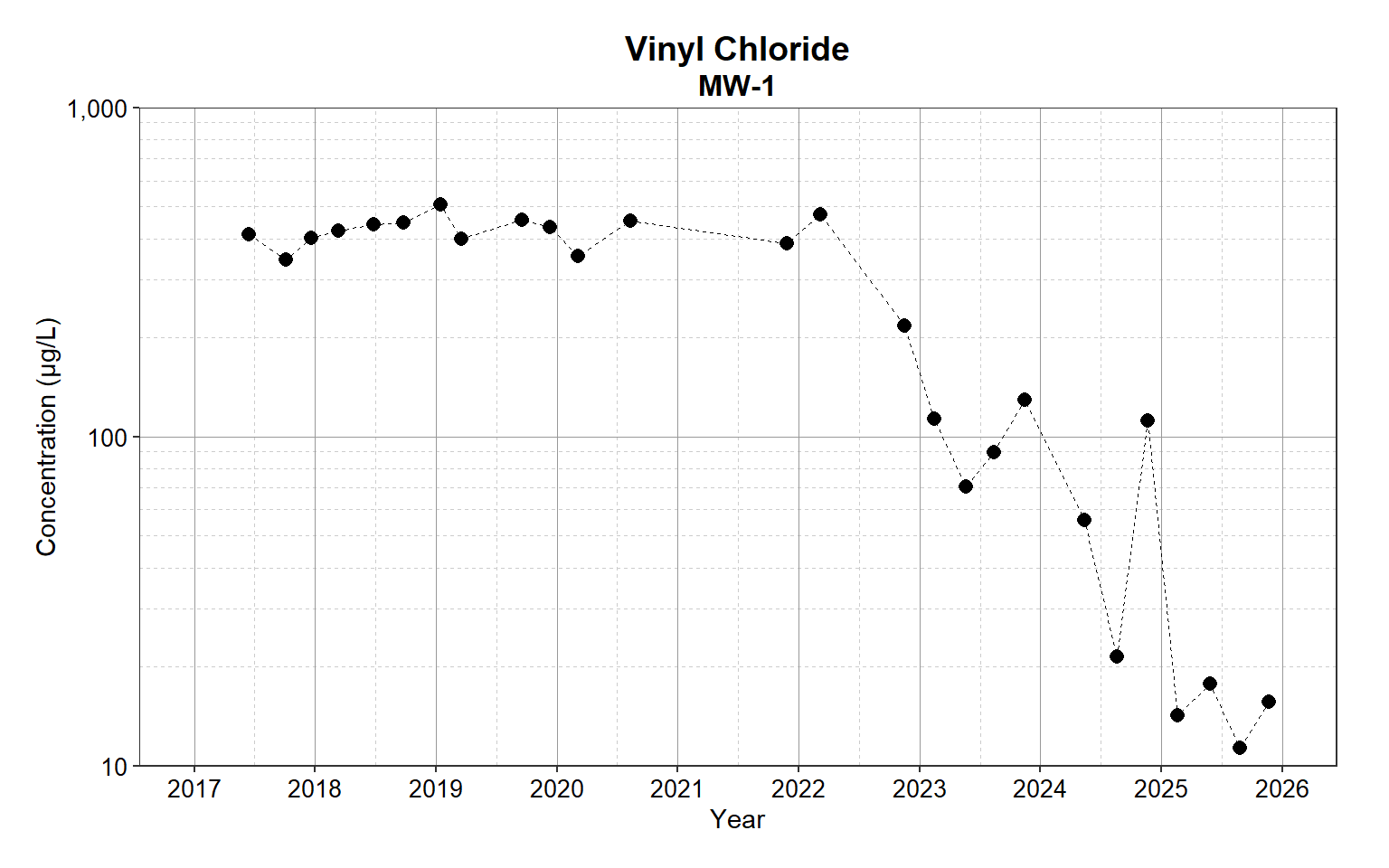
Shown below is a time-series plot for each vinyl chloride at well MW-1. In this plot, the measured concentrations are plotted against the sample collection dates. Time-series plots support statistical analysis by visually identifying the long-term direction of data, showing whether values are generally increasing, decreasing, or remaining stable. The plots also can be used to help identify seasonal or cyclical patterns in the data that may influence statistical analysis.

# Generate time-series plot
ts_plot(dat)

Single Linear Regression

The natural log-transformed data were regressed against sampling date. The results are presented below.

# Create dataframe of log-transformed data
df <- data.frame(x = dat$DATE, y = log(dat$RESULT))

# Fit a linear regression model to the log-transformed data
fit_lm <- lm(y ~ x, data = df)
summary(fit_lm)
## 
## Call:
## lm(formula = y ~ x, data = df)
## 
## Residuals:
##      Min       1Q   Median       3Q      Max 
## -1.03117 -0.59218  0.00869  0.32492  1.32020 
## 
## Coefficients:
##              Estimate Std. Error t value Pr(>|t|)    
## (Intercept) 811.72239   95.23914   8.523 1.01e-08 ***
## x            -0.39902    0.04711  -8.470 1.13e-08 ***
## ---
## Signif. codes:  0 '***' 0.001 '**' 0.01 '*' 0.05 '.' 0.1 ' ' 1
## 
## Residual standard error: 0.6698 on 24 degrees of freedom
## Multiple R-squared:  0.7493,	Adjusted R-squared:  0.7389 
## F-statistic: 71.74 on 1 and 24 DF,  p-value: 1.132e-08

# Get the intercept and slope for the loglinear model
coef(fit_lm)
## (Intercept)           x 
## 811.7223904  -0.3990154

# Plot the loglinear model
rs_plot(dat, fit_lm)

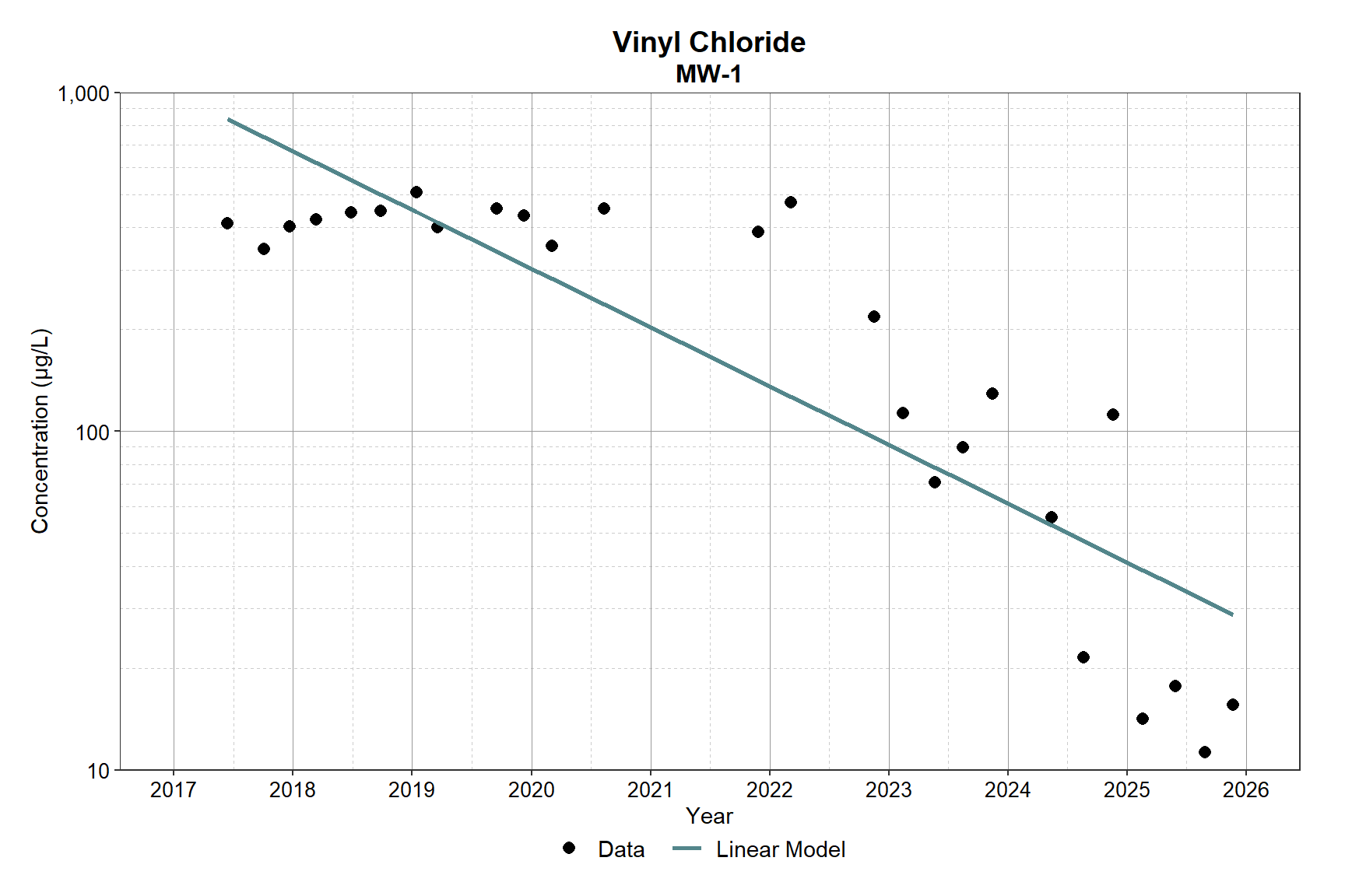
The linear regression reflects the overall downward trend in vinyl chloride concentrations but does not fully capture the variability in the data. Concentrations were relatively stable from 2017 to about 2022 despite the modeled decline, showed increased variability from 2022 to 2024, and then declined more sharply between 2024 and the end of 2025 than predicted by the model. Overall, the regression represents the general trend but does not account for apparent shifts and short-term fluctuations in the data.

Segmented Regression

A segmented regression using changepoint analysis was performed to improve the fit by identifying statistically significant shifts in trend (e.g., changes in slope). Prior to the segmented regression, Davies’ test (Davies 2002) was used to evaluate whether difference in slopes is significantly significant (i.e., is there a changepoint/breakpoint in the data). The null hypothesis is \(H0: \beta = 0\), where \(\beta\) is the difference-in-slopes The hypothesis of interest \(\beta = 0\) means no changepoint/breakpoint.

# Davies' test for difference in slopes
davies.test(fit_lm, k = 10)   # provide the lm() model
## 
## 	Davies' test for a change in the slope
## 
## data:  formula = y ~ x ,   method = lm 
## model = gaussian , link = identity  
## segmented variable = x
## 'best' at = 2022.1, n.points = 9, p-value = 6.688e-06
## alternative hypothesis: two.sided

The p-value <0.001, indicating that the null hypothese of no difference in slopes should be rejected (i.e., the data contain a changepoint/breakpoint). Because a structural break in the data was determined to be statistically significant, segmented regression was conducted to estimate separate slopes for each segment. A segmented regression evaluates the relationship between the response variable (y) and the explanatory variable (x) based on fitting piece-wise linear regressions that allow changes in the model at a changepoint/breakpoint. This results in interpretable models for each segment and can be used to identify thresholds where the relationship between the two variables changes (Muggeo 2003; Toms and Lesperance 2003). Depending on the context, a segmented model could have multiple changepoints/breakpoints.

# Fit a segmented regression model to the log-transformed data
fit_seg <- segmented(fit_lm, seg.Z = ~x, npsi = 1)
summary(fit_seg)
## 
## 	***Regression Model with Segmented Relationship(s)***
## 
## Call: 
## segmented.lm(obj = fit_lm, seg.Z = ~x, npsi = 1)
## 
## Estimated Break-Point(s):
##             Est. St.Err
## psi1.x 2022.035  0.398
## 
## Coefficients of the linear terms:
##               Estimate Std. Error t value Pr(>|t|)
## (Intercept)   1.444121 178.723142   0.008    0.994
## x             0.002274   0.088513   0.026    0.980
## U1.x         -0.918090   0.131611  -6.976       NA
## 
## Residual standard error: 0.3902 on 22 degrees of freedom
## Multiple R-Squared: 0.922,  Adjusted R-squared: 0.9114 
## 
## Boot restarting based on 6 samples. Last fit:
## Convergence attained in 2 iterations (rel. change 8.8452e-10)

# Get breakpoint and confidence interval around the breakpoint
fit_seg$psi
##        Initial     Est.    St.Err
## psi1.x      NA 2022.035 0.3981513
confint(fit_seg, level = 0.95)
##           Est. CI(95%).low CI(95%).up
## psi1.x 2022.03     2021.21    2022.86

The intercept and slope for each segment is shown below.

# Get the intercept and slope for each segment
intercept(fit_seg)
## $x
##                 Est.
## intercept1    1.4441
## intercept2 1857.9000
slope(fit_seg)
## $x
##             Est.  St.Err.   t value CI(95%).l CI(95%).u
## slope1  0.002274 0.088513  0.025691  -0.18129   0.18584
## slope2 -0.915820 0.097401 -9.402500  -1.11780  -0.71382

The segmented regression substantially improves the representation of the data by accounting for a clear structural change in concentration trends over time as shown in the regression plot below.

# Plot the segmented regression model
rs_plot(dat, fit_seg, m1_name = 'Segmented Model')

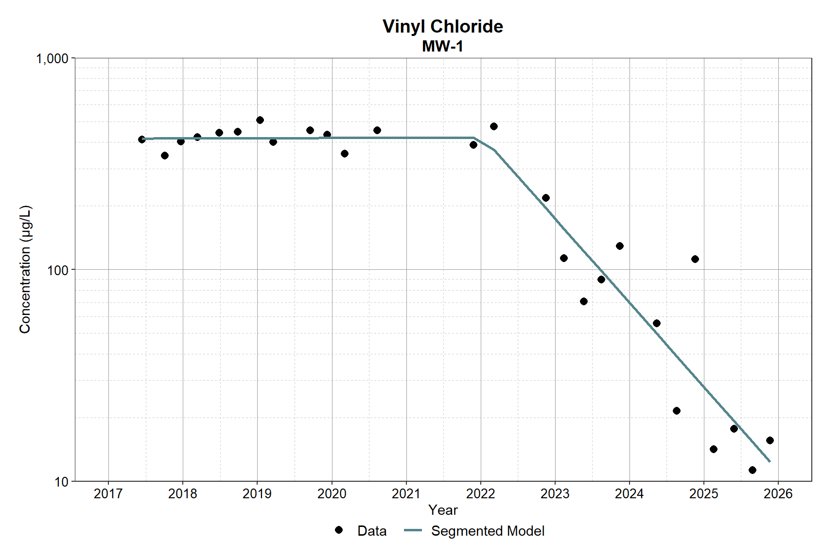
From approximately 2017 to early 2022, concentrations remain relatively stable in the 400 to 600 µg/L range. The segmented model reflects this behavior with an approximately flat slope during this period, closely matching the observed data and avoiding the artificial decline imposed by the single linear regression.

Around 2022, the model identifies a changepoint, after which concentrations decline sharply. The second segment captures the steep downward trend observed from 2022 through 2025, aligning much more closely with the rapid decrease in measured concentrations. This reduces the systematic overprediction seen in the later years under the single linear model.

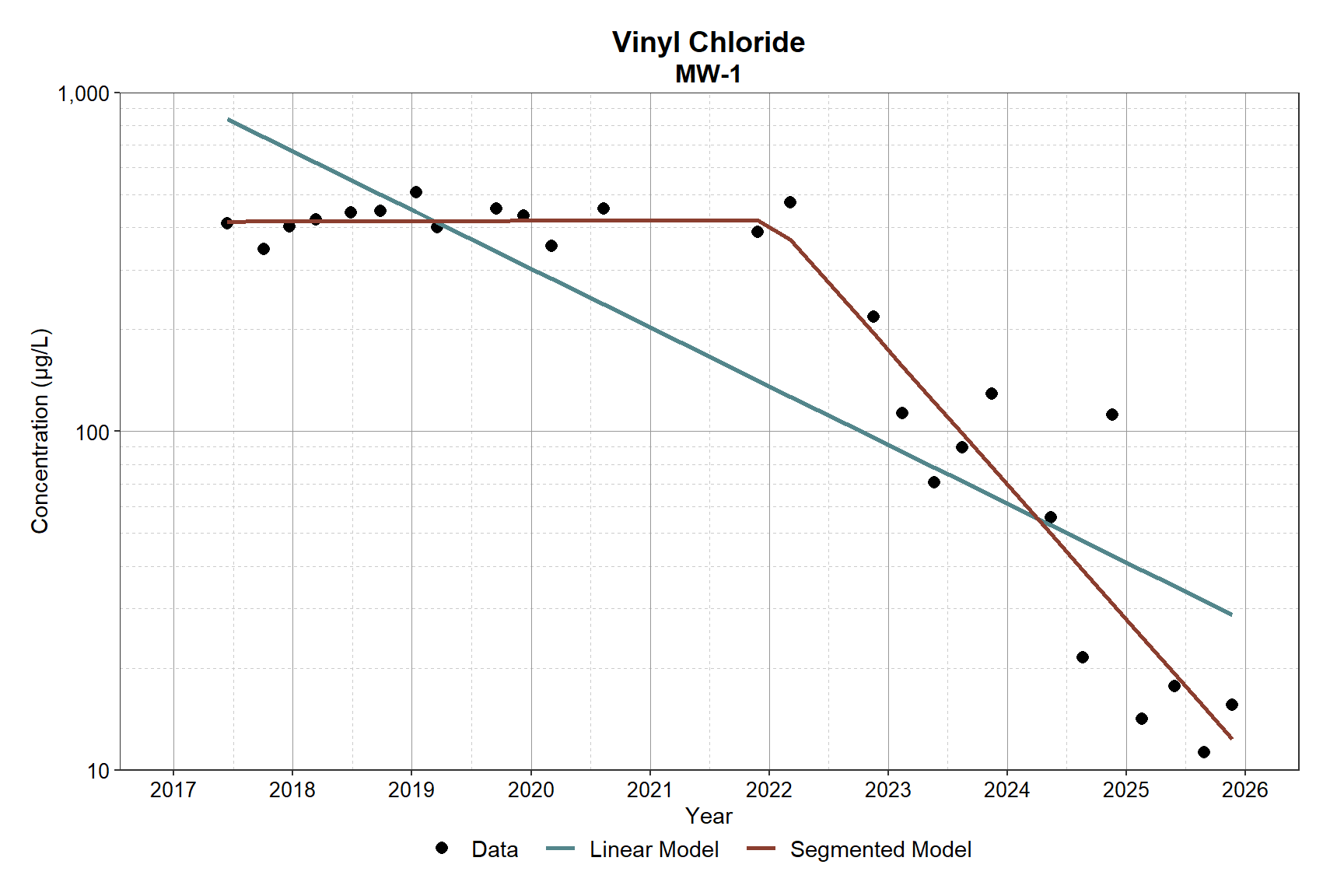
Below is a plot comparing the segmented regression model to the single linear model. The segmented regression model provides a better representation of the underlying behavior of vinyl chloride at MW-1, distinguishing between the distinct shift in concentration, providing a more accurate estimate of trend magnitude within each period. By allowing separate slopes before and after the changepoint, the model better reflects the underlying system behavior and provides a more realistic interpretation of temporal trends.

# Plot both tyh linear and segmented models
rs_plot(dat, fit_lm, fit_seg)

Remediation Timeframe Estimate

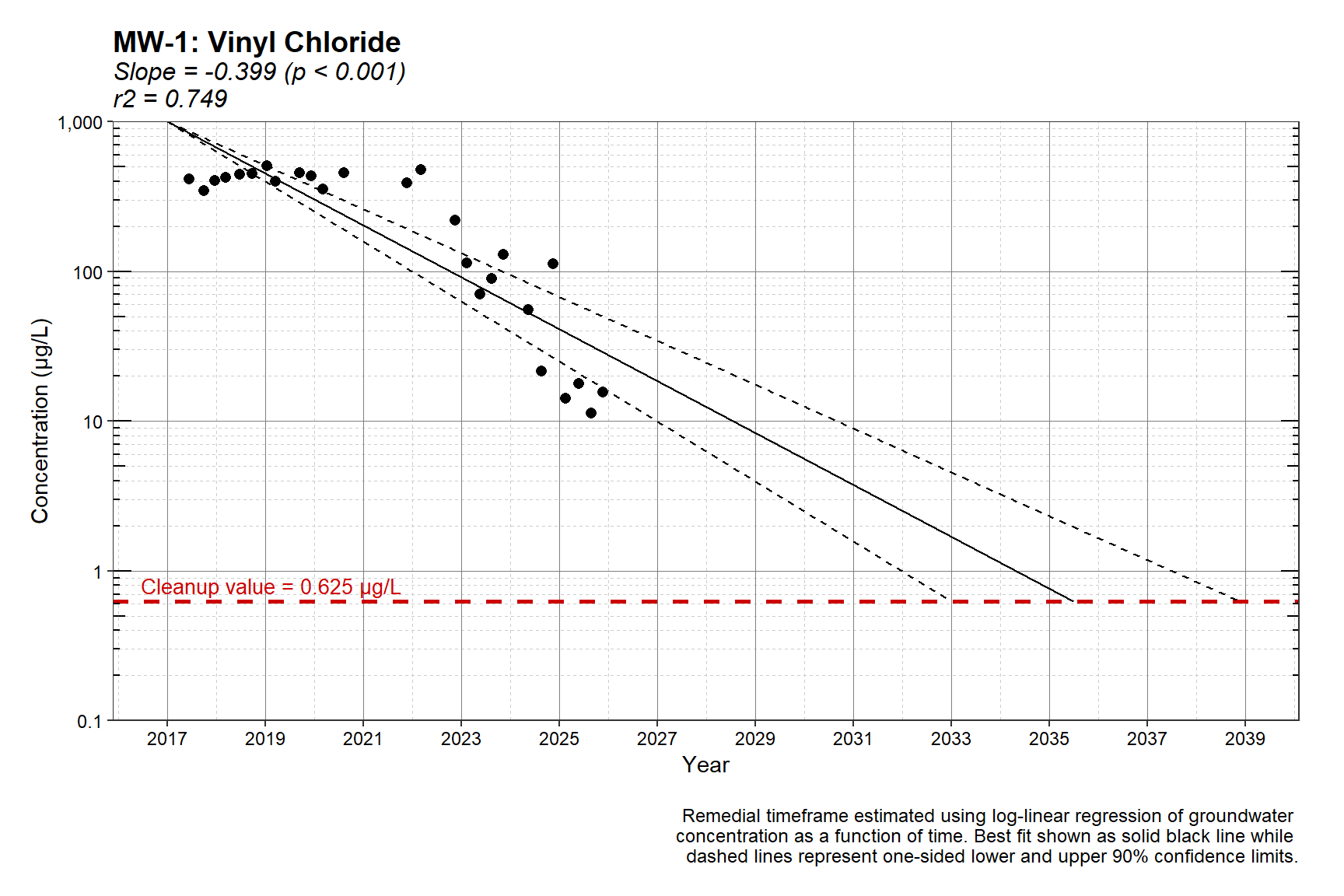
An estimate of the remediation timeframe for vinyl chloride at well MW-1 using the single linear regression model is shown below. The estimate assumes a cleanup goal of 0.625 µg/L. The best fit is shown as a solid black line while one-sided lower and upper 90% confidence limits are shown as dashed lines.

# Set confidence level and create cleanup levels
cf <- 0.80
clevels <- data.frame(PARAM = 'Vinyl Chloride', LEVEL = 0.625)

# Get remedial timeframe using loglinear regression
rdat <- rtf2(dat, clevels, cf)
rtf2_plot(dat, rdat)

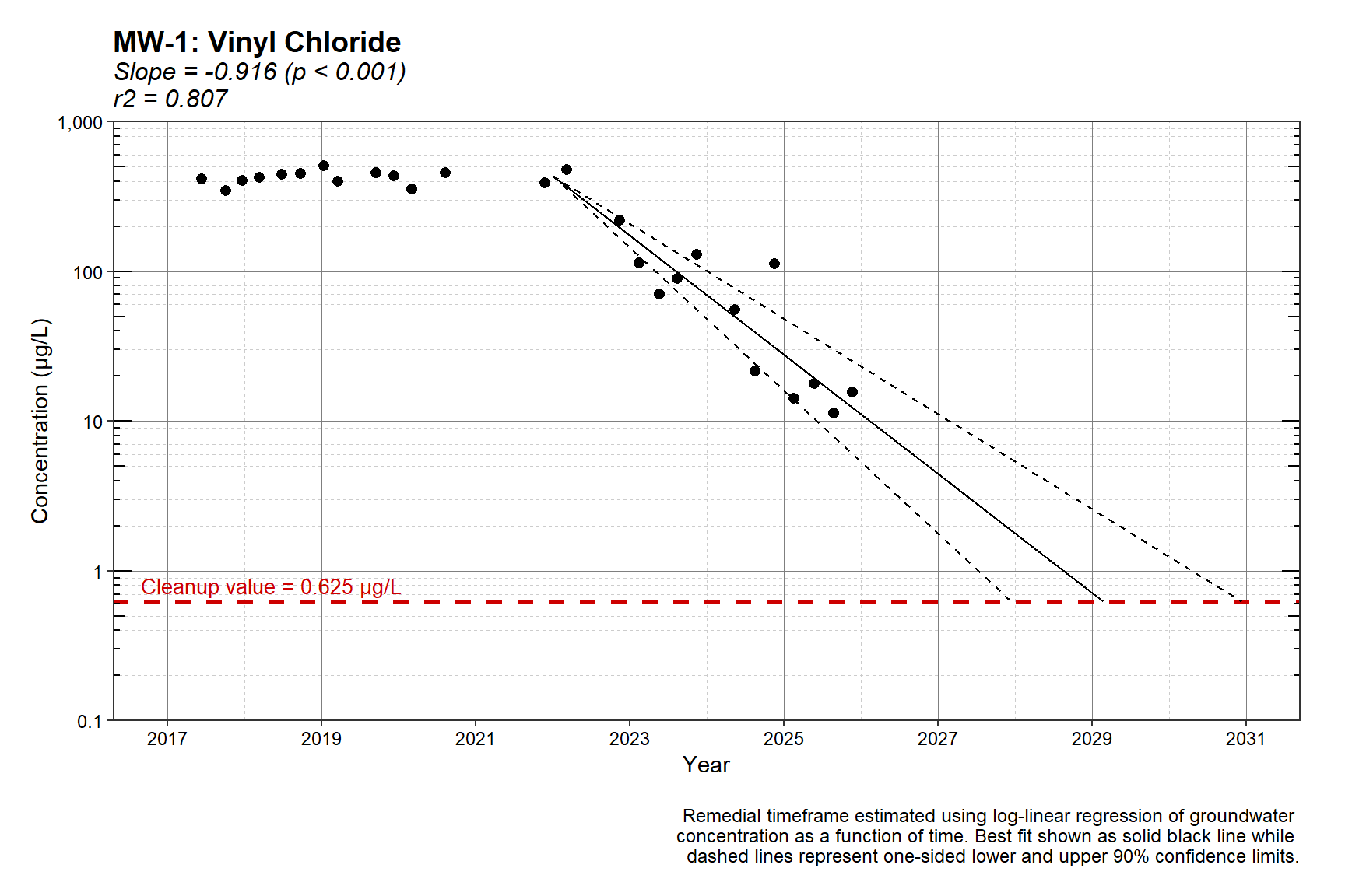
An estimate of the remediation timeframe for vinyl chloride at well MW-1 using the segmented regression model is shown below.

# Get remedial timeframe using changepoint
sdat <- dat %>% filter(DATE >= fit_seg$psi[2])
rdat2 <- rtf2(sdat, clevels, cf)
rtf2_plot(dat, rdat2)

The two plots show substantially different remediation timeframe estimates due to the modeling approach used. The single linear regression applies one continuous trend across the entire dataset (slope = -0.399, p<0.001; \(r^2\) = 0.749). Because it incorporates the relatively stable early-period data (2017-2021), the overall slope is moderated, resulting in a slower projected decline. As a result, the estimated time to reach the cleanup value of 0.625 µg/L extends to between approximately 2035 and 2039, depending on the confidence bound.

The segmented regression model isolates the post-changepoint decline (slope = -0.916, p<0.001; \(r^2\) = 0.807), excluding the earlier stable period from the slope calculation. This produces a much steeper decline that better reflects recent groundwater behavior. Consequently, the projected cleanup timeframe is significantly shorter, with attainment estimated between about 2028 and 2031, depending on the confidence bound.

Conclusions

Segmented regression provides a more accurate representation of vinyl chloride concentration in groundwater at well MW-1 by accounting for a clear changepoint around 2022. The model improves the analysis by accurately representing the stable early period, identifying and quantifying the timing of a significant trend shift, and providing a better fit to the steep decline in recent years. By allowing separate slopes before and after the changepoint, the model better reflects the underlying trends in groundwater concentration and provides a more realistic interpretation of temporal trends.

The single linear model yields a more conservative, longer remediation timeframe because it averages stable and declining periods into one trend. In contrast, the segmented regression better captures the structural shift in concentrations and produces a shorter, and likely more representative, remediation estimate based on current conditions.

References

Davies, R.B. 2002. Hypothesis Testing When a Nuisance Parameter is Present Only Under the Alternative: Linear Model Case. Biometrika 89, 484-489.

Ferrey, M.L., R.W. Bouchard Jr., and J.T. Wilson. 2024. Changepoint Analysis of Natural Attenuation in Groundwater Improves Forecasts of Time to Attain Goal. GWMR 44, 28-37.

Muggeo, V.M.R. 2003. Estimating Regression Models With Unknown Break-Points. Statistics in Medicine 22, 3055-3071.

Muggeo, V.M.R. 2006. Package segmented. https://cran.r-project.org/web/packages/segmented/segmented.pdf. January.

Newell, C.J., I. Cowie, T.M. McGuire, and W.W. McNab, Jr. 2006. Multiyear temporal changes in chlorinated solvent concentrations at 23 monitored natural attenuation sites. Journal of Environmental Engineering 132, 653-663.

R Core Team. 2025. R: A Language and Environment for Statistical Computing. R Foundation for Statistical Computing. Vienna, Austria. https://www.R-project.org.

Toms, J.D. and M.L. Lesperance. 2003. Piecewise Regression: A Tool for Identifying Ecological Thresholds. Ecology 84, 2034-2041.

United States Environmental Protection Agency (USEPA). 2002. Calculation and Use of First-Order Rate Constants for Monitored Natural Attenuation Studies. EPA/540/S-02/500. U.S. Environmental Protection Agency, Washington, D.C.

United States Environmental Protection Agency (USEPA). 2004. Performance Monitoring of MNA Remedies for VOCs in Ground Water. EPA 600/R-04/027. Office of Research and Development, National Risk Management Research Laboratory, U.S. Environmental Protection Agency, Ada, Oklahoma. April.