Introduction

The empirical variogram is commonly interpreted as a direct empirical representation of the underlying spatial covariance structure. However, its identifiability is fundamentally constrained by the sampling design. In particular, spatial variability occurring at scales smaller than the sampling interval cannot be resolved and contributes to the apparent nugget effect. This phenomenon is especially important in environmental contamination studies, where micro-scale heterogeneity can strongly influence risk assessment, remediation design, and kriging-based predictions.

This post formalizes the relationship between sampling resolution and variogram identifiability using the spectral representation of stationary random fields and the Matérn covariance family. We demonstrate mathematically how unresolved high-frequency (micro-scale) variability is absorbed into the nugget term and illustrate the effect using a Fast Fourier Transform (FFT)-based Matérn-like simulation. The results clarify why nugget variance cannot be interpreted solely as measurement error and emphasize the importance of aligning sampling design with expected spatial scales of variability.

Background

In environmental contamination studies, spatial prediction via kriging depends critically on the fitted variogram model. The variogram determines both the kriging weights and the kriging variance. In practice, the nugget parameter is often interpreted as measurement error or short-scale randomness. However, this interpretation can be misleading when sampling density is insufficient to resolve micro-scale spatial structure.

Consider a contaminated soil site exhibiting variability at multiple scales. Large-scale gradients may reflect transport mechanisms or deposition patterns, while fine-scale heterogeneity may arise from mixing processes, preferential pathways, or localized releases. If the sampling interval exceeds the correlation length of the fine-scale structure, the empirical variogram cannot resolve that structure. The resulting model may display a large nugget, reduced apparent spatial continuity, and altered effective range. These modeling artifacts directly affect kriging predictions and uncertainty quantification.

Understanding micro-scale variability is therefore essential when:

• designing sampling campaigns,
• interpreting nugget effects,
• selecting appropriate variogram models, and
• evaluating kriging-based decisions.

Mathematically, let \(Z(\mathbf{s})\), \(\mathbf{s} \in \mathbb{R}^2\), be a second-order stationary random field with covariance function:

\begin{equation}\tag{1} C(\mathbf{h}) = \mathrm{Cov}(Z(\mathbf{s}), Z(\mathbf{s}+\mathbf{h})) \end{equation}

where h is lag vector (distance and direction). The semivariogram is defined as:

\begin{equation}\tag{2} \gamma(\mathbf{h}) = \frac{1}{2}\mathrm{Var}\big[Z(\mathbf{s}) - Z(\mathbf{s}+\mathbf{h})\big] \end{equation}

Under stationarity, where the mean is constant and the covariance depends only on the separation h, not the absolute location s, this simplifies to the following:

\begin{equation}\tag{3} \gamma(\mathbf{h}) = C(0) - C(\mathbf{h}) \end{equation}

Thus, the variogram and covariance are equivalent second-order summaries (Cressie 1993; Chilès and Delfiner 2012). However, the empirical variogram is computed only at observed lag distances, which are determined by the sampling design.

Two-scale Decomposition and Identifiability

Assume the process decomposes into independent components given by:

\begin{equation}\tag{4} Z(\mathbf{s}) = Z_L(\mathbf{s}) + Z_M(\mathbf{s}) \end{equation}

where \(Z_L\) represents long-range structure and \(Z_M\) represents micro-scale variation.

Independence implies the following:

\begin{equation}\tag{5} C(\mathbf{h}) = C_L(\mathbf{h}) + C_M(\mathbf{h}) \end{equation}

and

\begin{equation}\tag{6} \gamma(\mathbf{h}) = \gamma_L(\mathbf{h}) + \gamma_M(\mathbf{h}) \end{equation}

If the micro-scale component has correlation length \(a_M\), then \(C_M(\mathbf{h})\) decays rapidly for \(\|\mathbf{h}\| \gg a_M\).

Suppose observations are collected on a regular grid with spacing h. The smallest observable lag is approximately h. If

\begin{equation}\tag{7} h > a_M \end{equation}

then no data pairs exist within the micro-scale range, and the curvature of \(C_M(\mathbf{h})\) near the origin cannot be estimated. For observed lags \(\|\mathbf{h}\| \ge h \gg a_M\),

\begin{equation}\tag{8} C_M(\mathbf{h}) \approx 0 \end{equation}

so that

\begin{equation}\tag{9} \gamma(\mathbf{h}) \approx \gamma_L(\mathbf{h}) + C_M(0) \end{equation}

By definition, the expected value of the squared deviation from the mean is the variance:

\begin{equation}\tag{10} C_M(0) = \mathrm{Var}(Z_M) \end{equation}

Thus, unresolved micro-scale variance appears as a near-origin discontinuity in the variogram and is empirically indistinguishable from nugget. Because \(C_M(\mathbf{h})\) vanishes almost immediately relative to the grid spacing h, the term \(C_M(0)\) acts as a mathematical constant added to all observable points. Even if the underlying physical process is continuous, the lack of data at forces the empirical variogram to “jump” at the origin to the first observed lag. The nugget is often not a measurement error, but rather unresolved spatial variance occurring at a scale smaller than the sampling density, a point emphasized in Stein (1999).

Spectral Representation and Matérn Structure

The Matérn covariance is a highly flexible class of spatial correlation models used in geostatistics. It is widely considered the “gold standard” because it generalizes other common models (like the Exponential and Gaussian) by adding a parameter that controls the smoothness of the random process. The Matérn structure is particularly useful for decomposition because unlike simpler models, the Matérn can model curvature near the origin when \(h \gt a_M\).

According to Bochner’s theorem, a stationary covariance can be defined through its spectral measure via a Fourier transform (Yaglom 1987):

\begin{equation}\tag{11} C(\mathbf{h}) = \int_{\mathbb{R}^2} e^{i\boldsymbol{\omega}\cdot\mathbf{h}} S(\boldsymbol{\omega}), d\boldsymbol{\omega} \end{equation}

where \(S(\boldsymbol{\omega})\) is the spectral density.

The Matérn covariance family has spectral density proportional to (Stein 1999):

\begin{equation}\tag{12} S(\omega) \propto (\kappa^2 + |\omega|^2)^{-(\nu + d/2)} \end{equation}

In two dimensions, this is given by:

\begin{equation}\tag{13} S(\omega) \propto (\kappa^2 + |\omega|^2)^{-(\nu + 1)} \end{equation}

The micro-scale variance \(\mathrm{Var}(Z_M)\) is the integral of the spectral density \(S(\boldsymbol{\omega})\) over the range of frequencies exceeding the Nyquist limit:

\begin{equation}\tag{14} \mathrm{Var}(Z_M) = \int_{|\omega| > \pi/h} S(\boldsymbol{\omega}), d\boldsymbol{\omega} \approx C_M(0) \end{equation}

Micro-scale variation corresponds to spectral mass at high frequencies. Sampling on a lattice with spacing h imposes a Nyquist-type frequency limit approximately equal to \(\pi/h\). Frequencies above this threshold cannot be uniquely resolved. Consequently, unresolved high-frequency variance contributes to \(C(0)\) but not to \(C(h)\) at observed lags, appearing as nugget in the variogram.

FFT-Based Matérn-Like Simulation

The following simulation illustrates how sampling interval controls what the empirical variogram can resolve. A single underlying field is as a stationary Gaussian random field by filtering white noise in the frequency domain using a Matérn-like amplitude spectrum. This avoids expensive covariance-matrix factorization and scales approximately as \(O(n\log n)\) due to the FFT (Dietrich and Newsam 1997).

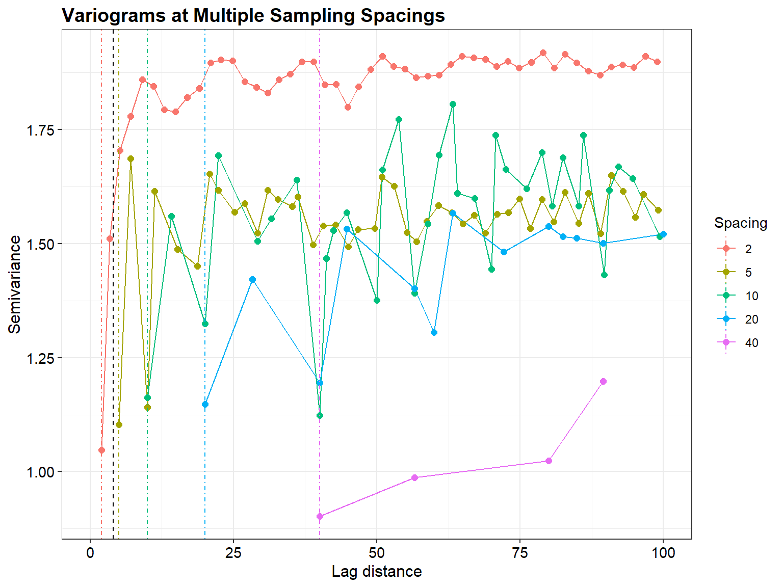
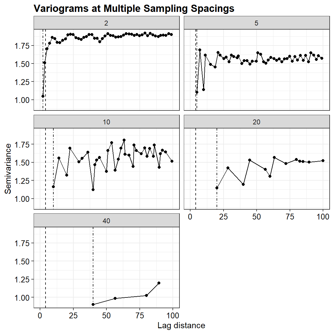
We simulate one underlying “truth” field on a fine grid, then sample that same field at multiple spacings and compute empirical variograms with identical binning. The plots include vertical reference lines indicating (i) the minimum resolvable lag (\(\approx\) spacing) and (ii) the micro-range (when included).

Packages and User Controls

library(sp)
library(gstat)
library(ggplot2)

set.seed(42)

L         <- 200
grid_step <- 1
use_micro <- TRUE

long_range  <- 80
micro_range <- 4

nu_long  <- 0.5
nu_micro <- 0.5

long_var  <- 1.0
micro_var <- 0.8

meas_nugget <- 0.0
spacings    <- c(2, 5, 10, 20, 40)

cutoff    <- 100
bin_width <- 2

Matérn-like FFT field generator

make_fft_field_matern <- function(nx, ny, dx, dy, range, nu = 0.5, var = 1.0) {

  kx <- if (nx %% 2 == 0) c(0:(nx/2), (-(nx/2-1)):-1) else c(0:((nx-1)/2), (-((nx-1)/2)):-1)
  ky <- if (ny %% 2 == 0) c(0:(ny/2), (-(ny/2-1)):-1) else c(0:((ny-1)/2), (-((ny-1)/2)):-1)

  fx <- kx / (nx * dx)
  fy <- ky / (ny * dy)

  wx <- 2 * pi * fx
  wy <- 2 * pi * fy

  wx2 <- matrix(rep(wx^2, times = ny), nrow = ny, byrow = TRUE)
  wy2 <- matrix(rep(wy^2, each  = nx), nrow = ny, byrow = FALSE)
  w2  <- wx2 + wy2

  d <- 2
  kappa <- sqrt(8 * nu) / range
  expo <- (nu + d/2) / 2
  A <- (kappa^2 + w2)^(-expo)

  w <- matrix(rnorm(nx * ny), nrow = ny, ncol = nx)

  W <- fft(w)
  Z <- fft(W * A, inverse = TRUE) / (nx * ny)
  z <- Re(Z)

  z <- z - mean(z)
  if (sd(z) > 0) z <- z / sd(z)

  z * sqrt(var)
}

Simulate underlying field

xs <- seq(0, L, by = grid_step)
ys <- seq(0, L, by = grid_step)
nx <- length(xs)
ny <- length(ys)

z_long  <- make_fft_field_matern(nx, ny, grid_step, grid_step,
                                 range = long_range, nu = nu_long, var = long_var)

z_micro <- if (use_micro) {
  make_fft_field_matern(
    nx, ny, grid_step, grid_step,
    range = micro_range, nu = nu_micro, var = micro_var
  )
} else 0

z <- z_long + z_micro

grid_df <- expand.grid(x = xs, y = ys)
grid_df$z <- as.vector(z)

coordinates(grid_df) <- ~ x + y

Empirical variogram

sample_field_regular <- function(sp_points, spacing) {
  df <- as.data.frame(sp_points)
  keep <- (df$x %% spacing == 0) & (df$y %% spacing == 0)
  s <- df[keep, c("x", "y", "z")]
  coordinates(s) <- ~ x + y
  s
}

samples_list <- lapply(spacings, function(h) {
  s <- sample_field_regular(grid_df, h)
  if (meas_nugget > 0)
    s$z <- s$z + rnorm(nrow(s), sd = sqrt(meas_nugget))
  s
})

compute_emp_variogram <- function(sp_points, cutoff, bin_width) {
  boundaries <- seq(0, cutoff, by = bin_width)
  variogram(z ~ 1, sp_points, cutoff = cutoff, boundaries = boundaries)
}

variograms <- lapply(samples_list, compute_emp_variogram,
                     cutoff = cutoff, bin_width = bin_width)

vdf <- do.call(rbind, lapply(seq_along(variograms), function(i) {
  v <- variograms[[i]]
  v$spacing <- spacings[i]
  v
}))

minlag_df <- data.frame(spacing = spacings, xintercept = spacings)
microrange_df <- data.frame(spacing = spacings, xintercept = micro_range)

Variogram plots with resolution markers

ggplot(vdf, aes(x = dist, y = gamma, color = factor(spacing))) +
  geom_line() +
  geom_point(size = 2) +
  geom_vline(data = minlag_df,
             aes(xintercept = xintercept, color = factor(spacing)),
             linetype = "dotdash", inherit.aes = FALSE) +
  geom_vline(data = microrange_df,
             aes(xintercept = xintercept),
             linetype = "dashed", inherit.aes = FALSE) +
  coord_cartesian(xlim = c(0, cutoff)) +
  labs(title = "Variograms at Multiple Sampling Spacings",
       x = "Lag distance",
       y = "Semivariance",
       color = "Spacing") +
  theme_bw() +
  theme(plot.title = element_text(margin = margin(b = 3), size = 14,
                       color = 'black', face = 'bold'),
        axis.title = element_text(size = 12, color = 'black'),
        axis.text = element_text(size = 11, color = 'black'))

Faceted variogram plots

ggplot(vdf, aes(x = dist, y = gamma)) +
  geom_line() +
  geom_point() +
  geom_vline(data = minlag_df,
             aes(xintercept = xintercept),
             linetype = "dotdash", inherit.aes = FALSE) +
  geom_vline(data = microrange_df,
             aes(xintercept = xintercept),
             linetype = "dashed", inherit.aes = FALSE) +
  facet_wrap(~ spacing, ncol = 2, scales = "fixed") +
  coord_cartesian(xlim = c(0, cutoff)) +
  labs(title = "Variograms at Multiple Sampling Spacings",
       x = "Lag distance",
       y = "Semivariance",
       color = "Spacing") +
  theme_bw() +
  theme(plot.title = element_text(margin = margin(b = 3), size = 13,
                       color = 'black', face = 'bold'),
        axis.title = element_text(size = 11, color = 'black'),
        axis.text = element_text(size = 10, color = 'black'))

Sampling locations

samp_plot_df <- do.call(rbind, lapply(seq_along(samples_list), function(i) {
  s <- as.data.frame(samples_list[[i]])
  s$spacing <- spacings[i]
  s
}))

ggplot(samp_plot_df, aes(x = x, y = y)) +
  geom_point(size = 0.7, alpha = 0.85) +
  coord_equal() +
  facet_wrap(~ spacing, ncol = 3) +
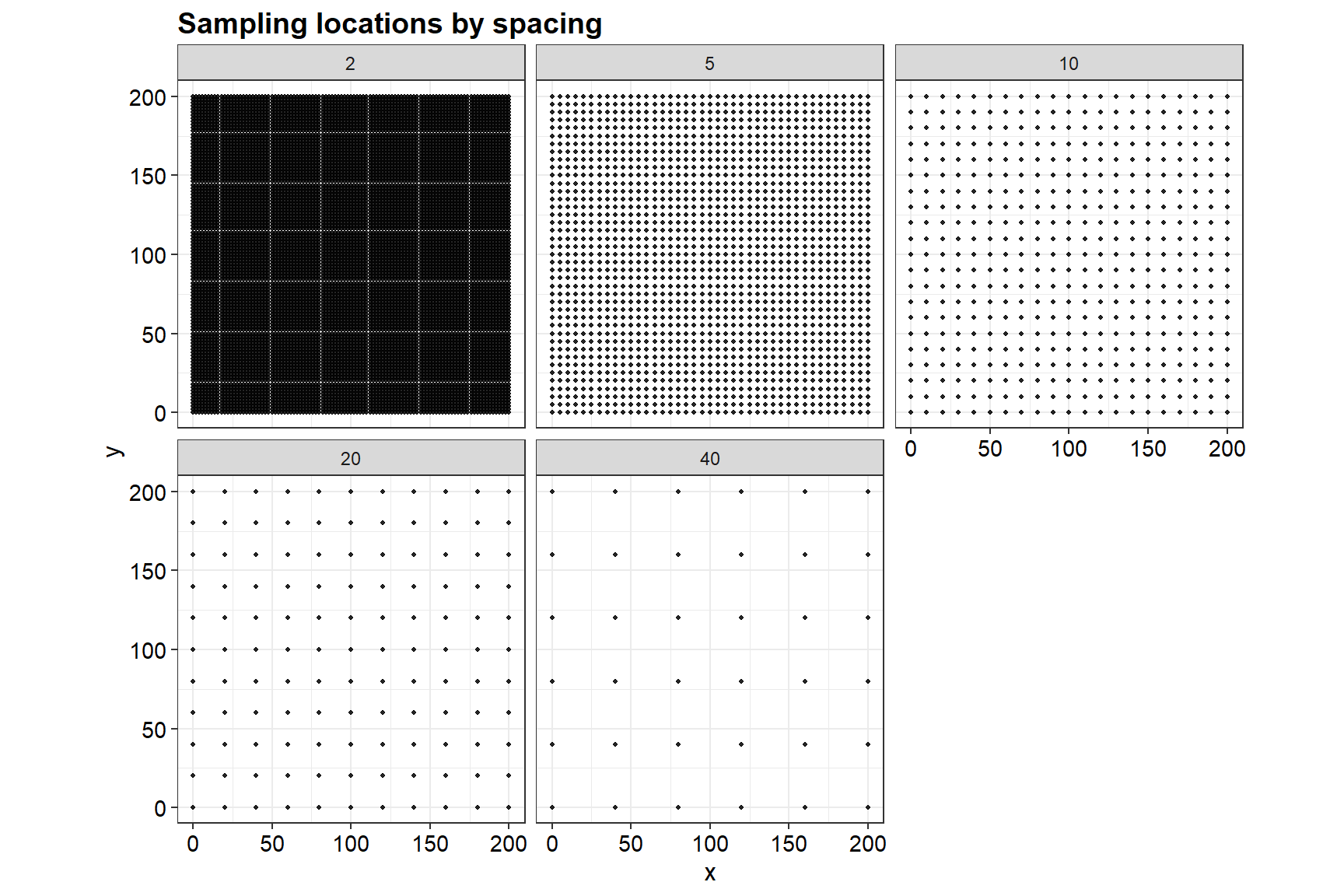
  labs(title = "Sampling locations by spacing", x = "x", y = "y") +
  theme_bw() +
  theme(plot.title = element_text(margin = margin(b = 3), size = 14,
                       color = 'black', face = 'bold'),
        axis.title = element_text(size = 12, color = 'black'),
        axis.text = element_text(size = 11, color = 'black'))

Nugget Inflation and Kriging Variance

The kriging predictor at location \(\mathbf{s}_0\) can be written as

$$\hat{Z}(\mathbf{s}_0) = \sum_{i=1}^{n} \lambda_i Z(\mathbf{s}_i)\tag{15}$$

where the weights \(\lambda_i\) are determined by the covariance (or variogram) model. The ordinary kriging variance is

$$\sigma_K^2(\mathbf{s}_0) = C(0) - \mathbf{c}^\top \mathbf{C}^{-1} \mathbf{c} + \frac{\left(1 - \mathbf{1}^\top \mathbf{C}^{-1} \mathbf{c}\right)^2}{\mathbf{1}^\top \mathbf{C}^{-1} \mathbf{1}}\tag{16}$$

where:

• \(\mathbf{C}\) is the covariance matrix among sampled locations,
• \(\mathbf{c}\) is the covariance vector between \(\mathbf{s}_0\) and sampled locations,
• \(\mathbf{1}\) is a vector of ones.

When unresolved micro-scale variability inflates the nugget term, \(C(0)\) increases while off-diagonal covariances remain largely unchanged at observed lags. This has two important consequences. First, diagonal dominance of \(\mathbf{C}\) increases, which reduces spatial influence among neighboring observations and shifts kriging weights toward more local averaging. Second, the kriging variance increases because \(C(0)\) enters directly into the expression for \(\sigma_K^2(\mathbf{s}_0)\). Even if the underlying physical process has strong short-range continuity, failure to resolve micro-scale structure produces larger reported prediction uncertainty.

Thus, nugget inflation due to coarse sampling not only alters the fitted variogram, but also directly affects:

• kriging weights,
• smoothing behavior,
• and reported prediction variance.

In environmental contamination studies, this can materially affect delineation of contaminated zones, compliance decisions, and remediation cost estimates. Proper interpretation of nugget therefore requires understanding whether it reflects measurement error, true discontinuity, or unresolved spatial variability.

Numerical Illustration: Nugget Inflation

The discussion above can be made concrete with a small numerical experiment. We take one sampled dataset (here, a coarser spacing) and compute ordinary kriging variances under two fixed covariance models with the same total variance:

1. A model that includes an explicit micro-scale component (short range, small nugget).
2. A model where the same micro-scale variance is instead assigned to the nugget (inflated nugget).

Because the nugget contributes directly to \(C(0)\) (and hence the kriging variance expression), the inflated-nugget model typically produces larger kriging variances. This is shown below in a numerical illustration.

# Choose one sampling spacing for the illustration (coarser = stronger effect)
spacing_demo <- 20
idx <- which(spacings == spacing_demo)
stopifnot(length(idx) == 1)

samp <- samples_list[[idx]]

# Prediction grid (coarser than the simulation grid for speed)
pred_step <- 5
pred_df <- expand.grid(
  x = seq(0, L, by = pred_step),
  y = seq(0, L, by = pred_step)
)
coordinates(pred_df) <- ~ x + y

# Define two covariance (variogram) models with the same total variance.

# (A) explicit micro-scale structure: long-range + micro-scale (nested), no nugget
model_micro <- vgm(psill = long_var,  model = "Exp", range = long_range,  nugget = 0)
model_micro <- rbind(model_micro, vgm(psill = micro_var, model = "Exp", range = micro_range, nugget = 0))

# (B) nugget-inflated model: same long-range, but micro-scale variance moved into nugget
model_nugget <- vgm(psill = long_var, model = "Exp", range = long_range, nugget = micro_var)

# Ordinary kriging variances under each model
ok_micro  <- krige(z ~ 1, locations = samp, newdata = pred_df, model = model_micro)
## [using ordinary kriging]
ok_nugget <- krige(z ~ 1, locations = samp, newdata = pred_df, model = model_nugget)
## [using ordinary kriging]

# Extract kriging variances
v_micro  <- ok_micro$var1.var
v_nugget <- ok_nugget$var1.var

# Summarize
summary_df <- data.frame(
  model = c("Explicit micro-scale", "Inflated nugget"),
  mean  = c(mean(v_micro), mean(v_nugget)),
  median= c(median(v_micro), median(v_nugget)),
  p90   = c(quantile(v_micro, 0.90), quantile(v_nugget, 0.90)),
  max   = c(max(v_micro), max(v_nugget))
)

Shown below is a plot of the kriging variance under the two models. The inflated nugget model (shown in blue), treats micro-scale variance as a “jump” at the origin. The explicit micro-scale model (shown in red) attempts to model the micro-scale component as a spatially correlated process, even though its range is smaller than the sampling spacing.

plot_df <- data.frame(
  var = c(ok_micro$var1.var, ok_nugget$var1.var),
  model = factor(
    rep(c("Explicit micro-scale", "Inflated nugget"),
        each = nrow(ok_micro)),
    levels = c("Explicit micro-scale", "Inflated nugget")
  )
)

ggplot(plot_df, aes(x = var, fill = model)) +
  geom_histogram(bins = 40, alpha = 0.7, position = "identity") +
  labs(
    title = paste0(
      "Kriging variance under two models (sampling spacing = ", spacing_demo, ")"
    ),
    subtitle = paste0(
      "Same total variance; micro-scale variance is either modeled explicitly\n",
      "or absorbed into the nugget"
    ),
    x = "Kriging variance",
    y = "Count",
    fill = "Model"
  ) +
  theme_bw() +
  theme(plot.title = element_text(margin = margin(b = 3), size = 13,
                       color = 'black', face = 'bold'),
        plot.subtitle = element_text(margin = margin(b = 3), size = 11,
                       color = 'black'),
        axis.title = element_text(size = 12, color = 'black'),
        axis.text = element_text(size = 11, color = 'black'),
        legend.title = element_text(size = 12),
        legend.text = element_text(size = 11))

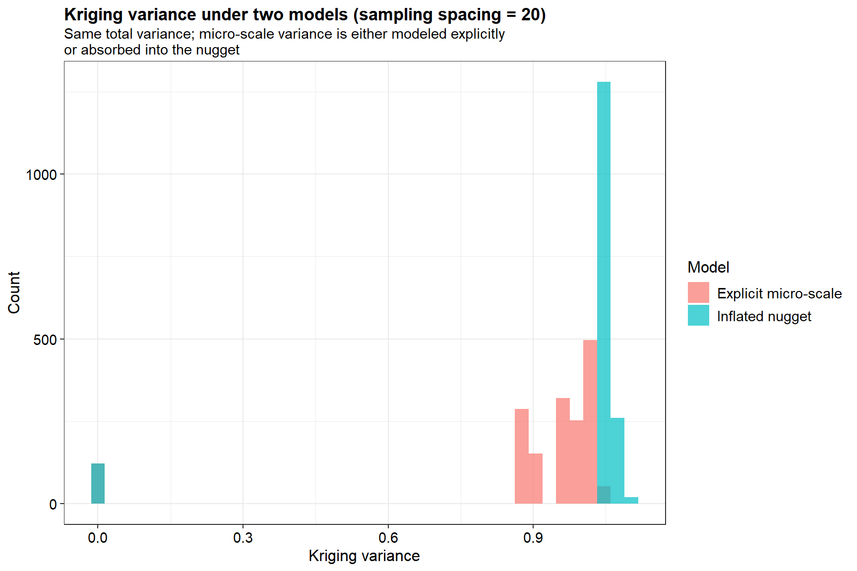
The inflated nugget model shows a very narrow, tall spike of kriging variances near 1. This indicates that the uncertainty is consistently high and relatively constant across the study area because the model can’t resolve local detail, treating it as random noise. The explicit micro-scale model has a wider, more spread-out distribution of variances. By trying to model the structure of the micro-scale variation, the kriging equations produce different levels of uncertainty depending on how close a prediction point is to an observation, even within that “micro” range.

While the two models have the same total variance, they produce different predictive distributions. The inflated nugget model is more conservative; it treats unresolved variation as irreducible noise. The explicit model tries to “smooth” the noise, which results in the varying (red) bars. Treating unresolved micro-scale variation as a nugget leads to a more “honest” but generally higher and more uniform estimate of prediction error when the sampling grid is too coarse.

Conclusions

The preceding derivations and simulations demonstrate that the empirical variogram reflects both the underlying spatial process and the sampling design. When sampling intervals exceed micro-scale correlation lengths, fine-scale variability can not be estimated and is absorbed into the nugget term. The practical consequence is nugget inflation. When short-range structure is not directly observable, its variance contribution is absorbed into the nugget parameter. This affects not only the visual appearance of the variogram, but also the behavior of kriging. Nugget inflation increases kriging variance and alters the weighting structure, leading to stronger smoothing and larger reported prediction uncertainty.

For environmental contamination studies, decisions regarding exposure risk, cleanup thresholds, and delineation of contaminated zones often rely on kriging predictions and associated uncertainty estimates. If micro-scale variability is unresolved due to coarse sampling, the fitted variogram may misrepresent true spatial continuity, and kriging-based decision metrics may shift accordingly. Designing sampling campaigns without regard to plausible short-scale variability may lead to systematic underestimation of spatial continuity and overestimation of prediction uncertainty.

The findings presented here offer several key insights:

• Sampling design must be informed by plausible spatial scales of variability. If fine-scale heterogeneity is expected, pilot sampling at higher density may be necessary to identify its magnitude and range.

• Interpretation of nugget should be cautious. Nugget represents the sum of measurement error and any unresolved spatial variability. Distinguishing these components requires either replicated measurements or multi-scale sampling strategies.

• Comparisons across sites or datasets should account for sampling resolution. Apparent differences in nugget or effective range may reflect differences in sampling density rather than intrinsic differences in spatial structure.

In summary, the variogram is an interface between stochastic structure and observational design. Recognizing this interplay is essential for responsible variogram modeling, accurate kriging, and defensible environmental decision-making.

References

Chilès, J.P. and P. Delfiner. 2012. Geostatistics: Modeling Spatial Uncertainty (2nd ed.). Wiley.

Cressie, N. (1993). Statistics for Spatial Data (Revised ed.). Wiley.

Dietrich, C.R. and G.N. Newsam. 1997. Fast and exact simulation of stationary Gaussian processes through circulant embedding of the covariance matrix. SIAM Journal on Scientific Computing, 18, 1088-1107.

Stein, M.L. 1999. Interpolation of Spatial Data: Some Theory for Kriging. Springer.

Yaglom, A.M. 1987. Correlation Theory of Stationary and Related Random Functions (Vol. I). Springer.