Species Distribution Modelling of Bigfoot Encounters Across North America
By Charles Holbert
October 12, 2022
Introduction
Understanding and predicting geographic and environmental distributions of species is an important application in quantitative ecology. Correlative summaries of species’ environmental associations and the relationships of those associations to their geographic distributions generally are referred to as species distribution models (SDM), ecological niche models (ENM), habitat modelling, predictive habitat distribution modelling, and range mapping (Elith and Leathwick. 2009; Peterson and Soberon 2012; Hijmans and Elith 2017). These models use computer algorithms to predict the occurrence of species on a landscape from georeferenced site locality data and sets of spatially explicit environmental data layers that are assumed to correlate with the species’ range (Lozier et al. 2009). These models can be used to understand how environmental conditions influence the occurrence or abundance of a species. They also play an important role in studying the current and future impacts of global changes to species habitat and understanding the extinction rate in natural ecosystems (Franklin 2010).
The objective of this post is to provide a brief introduction to SDMs and to illustrate how machine learning can be used to predict the range of a species based on a set of locations where it has been observed. This examination is by no means an exhaustive review of all aspects associated with modelling the relationship between the presence of a species and environmental factors. Instead, this post introduces the basic concepts and demonstrates how a SDM can be developed using the SSDM library and the R programming language for statistics and data visualization.
Species Distribution Modelling
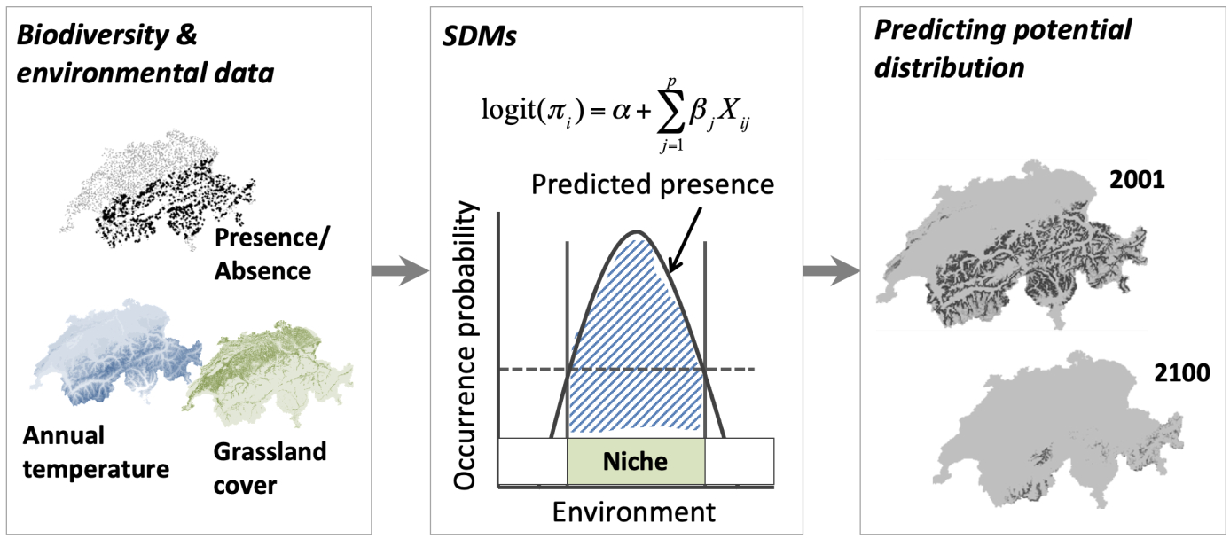
SDMs require georeferenced biodiversity observations, such as species presence/absence data, and geographic layers of environmental information data. These data are most often climate data (e.g., temperature and precipitation), but can include other variables such as soil type, water depth, and land cover. Different statistical and machine-learning algorithms are used to relate the biodiversity observations at specific sites to the prevailing environmental conditions at those sites. These biodiversity-environment relationships are then used to make predictions in space and in time by projecting the model onto available environmental layers. A conceptualization of species distribution modelling is shown in the figure below (Zurell 2020). In this conceptualization a generalized linear model is used to estimate the species-environment relationship. Many different statistical algorithms are available for modelling, and often several algorithms are combined into ensemble models, where a number of alternative statistical methods are used to explore the range of projections across the different SDMs.
Load Libraries
First, we’ll start by loading the libraries needed for this exercise.
# Load libraries
library(dplyr)
library(ggplot2)
library(geodata)
library(stars)
library(SSDM)
library(raster)
library(sf)
library(rnaturalearth)
Data Inputs
SDMs work on the principle of the likelihood of species occurrences at a spatial location using environmental variables, thus quantifying the environmental conditions that may lead to species occurrence. The models require species occurrence points (longitude and latitude) and environmental or bioclimatic characteristics of each of those occurrence points as inputs.
Species
Let’s use SDMs to predict the range of a crypto-zoological species - the North American Sasquatch, otherwise known as Bigfoot. Bigfoot is regularly reported in forested lands of western North America, as well as being considered a significant indigenous American and western North American folk legend (Meldrum 2007). The existence of this creature has never been verified with a typed specimen. In fact, this species is so hard to find that its very existence is commonly denied by mainstream media.
The data consists of over 4,200 reported Bigfoot encounters across North America between January 1921 and August 2022 archived by the Bigfoot Field Researchers Organization (BFRO). The BFRO has compiled a detailed database of Bigfoot sightings going back to the 1920s. Each sighting is dated, located to the nearest town or road, and contains a full description of the sighting. All reports posted into the BFRO’s online database are assigned a classification: Class A, Class B, or Class C. Class A reports involve clear sightings in circumstances where misinterpretation or misidentification of other animals can be ruled out with greater confidence. Class B reports involve sightings at great distances, in poor lighting conditions, or in any other circumstance that did not afford a clear view. Class C reports involve second-hand reports, and any third-hand reports, or stories with an untraceable source.
Let’s load the reported Bigfoot encounters data.
# Load bigfoot sightings data
bigfoot_data <- read.csv('./data/bigfoot.csv', header = T)

# Inspect structure of data
str(bigfoot_data)
## 'data.frame':	4273 obs. of  4 variables:
##  $ LONG : num  -79.7 -121.9 -86.1 -101.3 -83.5 ...
##  $ LAT  : num  36.9 49.2 46 48.3 35.7 ...
##  $ CLASS: chr  "A" "A" "A" "A" ...
##  $ DATE : chr  "8/15/1985" "3/2/2006" "4/1/1962" "4/21/2000" ...
Environmental Variables
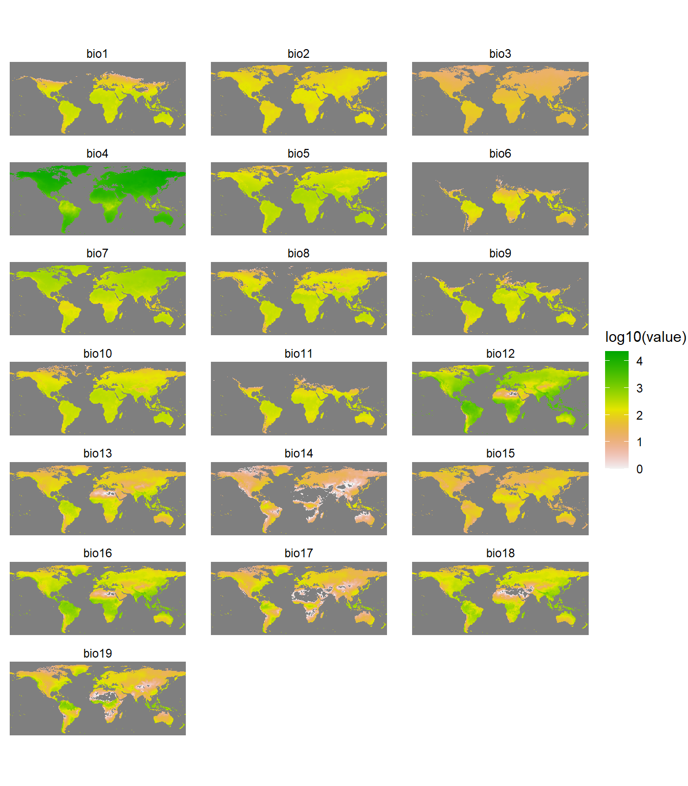
Distributions of species are affected by diverse factors (Udvardy 1969; Brown and Lomolino 1998; Gaston 2003), including history, environments, interactions with other species, dispersal capacity, and dispersal barriers (Peterson et al. 2011). For simplicity, we will use climate data. Specifically, we will use environmental data layers constructed for the 19 bioclimatic (BIOCLIM) variables (at 10-arcminute resolution) in the WORLDCLIM dataset (Hijmans et al. 2005). The BIOCLIM variables represent annual trends (e.g., mean annual temperature, annual precipitation), seasonality (e.g., annual range in temperature and precipitation), and extreme or limiting environmental factors (e.g., temperature of the coldest and warmest month, and precipitation of the wet and dry quarters). They are coded as follows, where temperature data are in units of °C * 10 and precipitation data are in millimeter (mm):
BIO1 = Annual Mean Temperature
BIO2 = Mean Diurnal Range (Mean of monthly (max temp - min temp))
BIO3 = Isothermality (BIO2/BIO7) (* 100)
BIO4 = Temperature Seasonality (standard deviation *100)
BIO5 = Max Temperature of Warmest Month
BIO6 = Min Temperature of Coldest Month
BIO7 = Temperature Annual Range (BIO5 - BIO6)
BIO8 = Mean Temperature of Wettest Quarter
BIO9 = Mean Temperature of Driest Quarter
BIO10 = Mean Temperature of Warmest Quarter
BIO11 = Mean Temperature of Coldest Quarter
BIO12 = Annual Precipitation
BIO13 = Precipitation of Wettest Month
BIO14 = Precipitation of Driest Month
BIO15 = Precipitation Seasonality (coefficient of variation)
BIO16 = Precipitation of Wettest Quarter
BIO17 = Precipitation of Driest Quarter
BIO18 = Precipitation of Warmest Quarter
BIO19 = Precipitation of Coldest Quarter
Let’s load the bioclimatic data. The data can be directly downloaded with R using the getData() function in the raster library. However, let’s load the individual files from a previous download and then create a RasterStack using the stack() function in the raster library.
# Load bioclimatic data
files <- NULL
for(i in 1:19) {
  f <- paste0(getwd(), '/data/wc10/', 'bio', i, '.bil')
  files <- c(files, f)
}
wc <- raster::stack(files)
Let’s quickly inspect the environmental variables using the gplot() function in the rasterVis library. The gplot() function is a wrapper function around the ggplot2 library.
# Plot rasters
library(rasterVis)
gplot(wc) +
  geom_tile(aes(fill = log10(value))) +
  facet_wrap(~ variable, ncol = 3) +
  scale_fill_gradientn(colors = rev(terrain.colors(225))) +
  coord_equal() +
  theme_void() +
  theme(plot.margin = margin(l = 1, r = 1, b = 1, t = 1))
Crop Environmental Rasters
Let’s use a background map of the continental United States that includes the 48 contiguous states but not Alaska, Hawaii, Puerto Rico, and the other U.S. territories to crop the environmental raster files. We can import a shapefile of the states using the tigris library. The tigris library allows users to directly download and use TIGER/Line shapefiles from the US Census Bureau. Let’s reproject the final shapefile into NAD 1983 Lambert North America for plotting.
# Extract borders of all US states
states <- tigris::states(cb = TRUE, progress_bar = FALSE) %>%
  dplyr::filter(
    !grepl(x = NAME, pattern = 'Puerto Rico|Hawaii|Mariana|Samoa|Virgin Islands|Guam')
  )

# Lower 48 states
lower48_geo <- states %>%
  filter(NAME != 'Alaska') %>%
  summarise() %>%
  sf::st_simplify(dTolerance = 1000)

# Crop out the parts of Alaska that cross the date line
lower48_geo <- lower48_geo %>%
  sf::st_crop(
    xmin = -180, ymin = 0,
    xmax = -40, ymax = 85
  )

# Reproject into NAD 1983 Lambert North America
lower48_proj <- lower48_geo %>%
  sf::st_transform('ESRI:102009')

# Crop environmental rasters to country borders or read saved output if exists
if (file.exists('./data/rasterstack_USA.RDS')) {

  rasterstack_USA <- readRDS('./data/rasterstack_USA.RDS')

} else {

  rasterstack_USA <- raster::mask(
    raster::crop(wc, lower48_geo), mask = lower48_geo
  ) %>%
  raster::projectRaster(crs = 'ESRI:102009')

  saveRDS(object = rasterstack_USA, file = './data/rasterstack_USA.RDS')
}
Convert Bigfoot Data
Let’s convert the bigfoot encounters data to a shapefile and then reproject the shapefile into NAD 1983 Lambert North America for plotting.
# Load bigfoot sightings data
bigfoot_data <- read.csv('./data/bigfoot.csv', header = T)

# Inspect structure of data
str(bigfoot_data)
## 'data.frame':	4273 obs. of  4 variables:
##  $ LONG : num  -79.7 -121.9 -86.1 -101.3 -83.5 ...
##  $ LAT  : num  36.9 49.2 46 48.3 35.7 ...
##  $ CLASS: chr  "A" "A" "A" "A" ...
##  $ DATE : chr  "8/15/1985" "3/2/2006" "4/1/1962" "4/21/2000" ...

# Prep bigfoot sightings data
sightings <- bigfoot_data %>%
  filter(!is.na(LONG) & !is.na(LAT)) %>%
  mutate(SPECIES = 'Biggus footus') %>%
  dplyr::select(SPECIES, LONGITUDE = LONG, LATITUDE = LAT) %>%
  sf::st_as_sf(., coords = c('LONGITUDE', 'LATITUDE')) %>%
  sf::st_set_crs('EPSG:4326') %>%
  sf::st_transform('ESRI:102009') %>%
  sf::st_filter(lower48_proj)
Now, let’s plot the reported Bigfoot encounters.
# Plot the encouters
ggplot() +
  geom_sf(data = states %>% filter(NAME != 'Alaska'), fill = NA,
          color = 'black', size = 0.2) +
  geom_sf(data = sightings, color = 'red') +
  labs(title = 'Bigfoot Sightings',
       caption = 'Data: Bigfoot Field Researchers Organization (bfro.net)') +
  coord_sf(crs = 'ESRI:102009', clip = 'off',
           xlim = c(-2227000, 2124000),
           ylim = c(-1528000, 1233000)) +
  theme_void() +
  theme(plot.title = element_text(size = 18, hjust = 0.5, margin = margin(b = 0),
                                  face = 'bold'),
        plot.caption = element_text(size = 9, color = 'black'),
        plot.margin = margin(l = 5, r = 5, b = 5, t = 5))
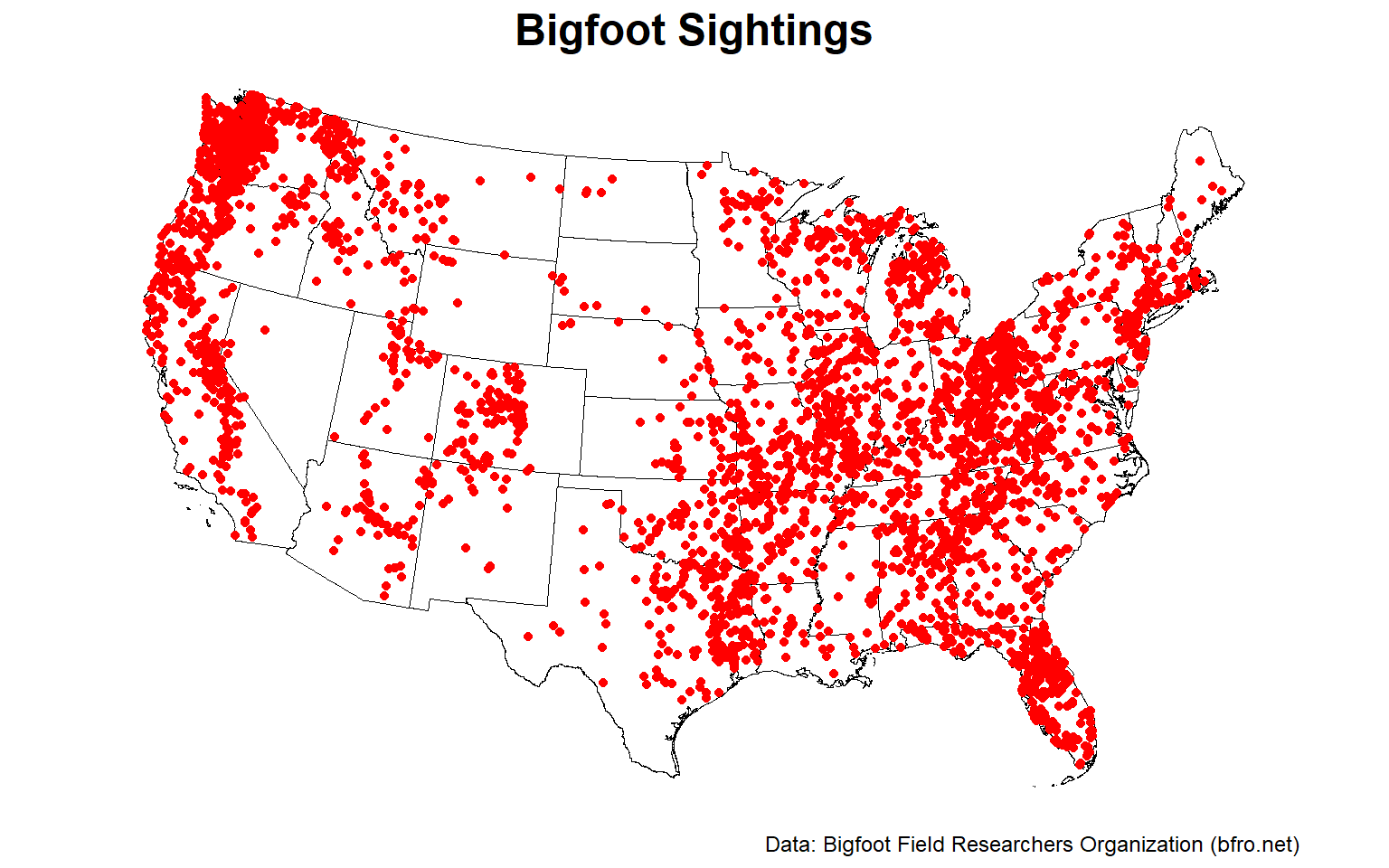
The pattern of encounters are not evenly distributed but appear clustered. There are distinct regions where encounters are incredibly common, likely due to terrain and habitat.
Plotting Functions
Prior to performing species distribution modelling, let’s create two functions to assist with plotting of the modelling results.
# Function to create plots
plotFunction <- function(x, main_title, title_size, cap, margin = FALSE,
                         type = 'prob', legend = TRUE, maxx = 1) {
  p <- ggplot() +
    geom_stars(data = x, na.action = na.omit) +
    geom_sf(data = states %>% filter(NAME != 'Alaska'), fill = NA,
            color = 'black', size = 0.2) +
    labs(title = main_title,
         caption = cap) +
    coord_sf(crs = 'ESRI:102009', clip = 'off',
             xlim = c(-2227000, 2124000),
             ylim = c(-1528000, 1233000)) +
    theme_void() +
    theme(plot.title = element_text(size = title_size, hjust = 0.5, margin = margin(b = 2),
                         face = 'bold'),
          plot.caption = element_text(size = 9, color = 'black'),
          legend.position = c(0.15, 0.15),
          legend.title = element_text(size = 10, lineheight = 1.1, face = 'bold'),
          legend.text = element_text(size = 9, lineheight = 1.1),
          legend.key.width = unit(1, units = 'cm'),
          legend.direction = 'horizontal')

  if (type == 'prob') {
    p <- p +
      scale_fill_gradient2(low = 'white', mid = '#FFFDAB', high = 'red', midpoint = maxx/2,
                           limits = c(0, maxx),
                           guide = guide_colorbar(nbin = 300,
                                                   frame.colour = 'black',
                                                   ticks = FALSE,
                                                   title.position = 'top', title.hjust = 0.5),
                           breaks = c(0, maxx),
                           labels = c('Low', 'High'),
                           name = 'Occurrence Probability')
  } else {
    p <- p +
      scale_fill_gradientn(colors = rev(terrain.colors(10)),
                           limits = c(0, maxx),
                           guide = guide_colorbar(nbin = 300,
                                                   frame.colour = 'black',
                                                   ticks = FALSE,
                                                   title.position = 'top', title.hjust = 0.5),
                           breaks = c(0, maxx),
                           labels = c('Low', 'High'),
                           name = 'Uncertainty')
  }

  if (margin == TRUE)
    p <- p + theme(plot.margin = margin(l = 10, r = 10, b = 5, t = 5))

  if (legend == FALSE)
    p <- p + theme(legend.position = 'none')

  return(p)
}

# Function to create plotting grid
place_plots <- function(p, legend_position) {

  st_list <- NULL
  for (i in 1:length(p)) {
    st <- paste0("p[[", i, "]] + theme(legend.position = 'none'),")
    st_list <- paste(st_list, st, sep = "\n")
  }
  st_list <- paste("cowplot::plot_grid(", st_list, "\nncol = 3)", sep = "\n")

  prow <- eval(parse(text = st_list))

  # Extract the legend from one of the plots
  legend <- cowplot::get_legend(
    p[[1]] + theme(legend.position = legend_position)
  )

  # Add the legend to the plots
  cowplot::plot_grid(prow, legend, ncol = 1, rel_heights = c(1, 0.1))
}
Species Distribution Modelling
The SSDM library includes several statistical methods for modelling species distributions. These methods include general additive models (GAD), generalized linear models (GLM), multivariate adaptive regression splines (MARS), classification tree analysis (CTA), generalized boosted models (GBM), maximum entropy (Maxent), artificial neural networks (ANN), random forests (RF), and support vector machines (SVM).
Differences between model projections may be significant. Therefore, let’s create an ensemble model combining outputs of several different SDMs. Let’s fit a number of alternative model algorithms, explore the range of projections across the different SDMs, and then produce a consensual map of occurrence. Two consensus methods are implemented in the SSDM library: (1) a simple average of the SDM outputs; and (2) a weighted average based on a user-specified metric or group of metrics. The SSDM library also creates an uncertainty map representing the between-algorithms variance. The degree of agreement between each pair of algorithms is assessed through a correlation matrix giving Pearson’s coefficient.
For our ensemble model, let’s combine four statistical algorithms: GLM, MARS, CTA, and RF. Let’s run 10 repetitions for each model using the area under the receiving operating characteristic (ROC) curve (AUC) for the ensemble metric with a threshold value of 0.7; only models with an AUC > 0.7 will be kept. For simplicity, let’s grow 100 trees for the RF model. Let’s also split the data into training and evaluation datasets using 70% as the training set and the remaining 30% as the evaluation set.
# Conduct species distribution modelling or read saved output if exists
if (file.exists('./data/ESDM_stars.RDS')) {

  ESDM_stars <- readRDS('./data/ESDM_stars.RDS')
  ESDM <- readRDS('./data/ESDM.RDS')

} else {

  # SSDM needs a df with coord cols for sightings
  sightings_df <- sightings %>%
    dplyr::bind_cols(sf::st_coordinates(.)) %>%
    dplyr::rename(LONGITUDE = X, LATITUDE = Y)

  # Run ensemble model using 3 different methods
  ESDM <- ensemble_modelling(
    c('GLM', 'MARS', 'CTA', 'RF'), trees = 100,
    Occurrences = sightings_df %>% sf::st_drop_geometry(),
    Env = rasterstack_USA,
    Xcol = 'LONGITUDE', Ycol = 'LATITUDE',
    ensemble.thresh = 0.7, rep = 10, verbose = FALSE
  )
  saveRDS(object = ESDM, file = './data/ESDM.RDS')

  # Convert output to stars because it's easier to plot when using ggplot
  ESDM_stars <- stars::st_as_stars(ESDM@projection)
  saveRDS(object = ESDM_stars, file = './data/ESDM_stars.RDS')
}
Now that we have built the model, let’s inspect the contents.
# Inspect model output
str(ESDM, max.level = 2)
## Formal class 'Ensemble.SDM' [package "SSDM"] with 11 slots
##   ..@ uncertainty          :Formal class 'RasterLayer' [package "raster"] with 12 slots
##   ..@ algorithm.correlation:'data.frame':	4 obs. of  4 variables:
##   ..@ algorithm.evaluation :'data.frame':	4 obs. of  8 variables:
##   ..@ sdms                 :List of 19
##   ..@ name                 : chr "Specie.Ensemble.SDM"
##   ..@ projection           :Formal class 'RasterLayer' [package "raster"] with 12 slots
##   ..@ binary               :Formal class 'RasterLayer' [package "raster"] with 12 slots
##   ..@ evaluation           :'data.frame':	1 obs. of  7 variables:
##   ..@ variable.importance  :'data.frame':	1 obs. of  19 variables:
##   ..@ data                 :'data.frame':	135885 obs. of  22 variables:
##   ..@ parameters           :'data.frame':	1 obs. of  12 variables:
The SSDM library provides two results in raster format: (1) a continuous raster map giving the probability of presence for presence/absence data; and (2) a binary presence/absence raster based on the threshold of habitat suitability that maximizes a user-specified accuracy metric. Additionally, the ensemble model includes a raster map of uncertainty representing the between-algorithms variance.
Individual SDMS
Let’s inspect the individual models that comprise the final ensemble model.
# Inspect model sdms output
str(ESDM@sdms, max.level = 2)
## List of 19
##  $ :Formal class 'GLM.SDM' [package "SSDM"] with 7 slots
##  $ :Formal class 'MARS.SDM' [package "SSDM"] with 7 slots
##  $ :Formal class 'MARS.SDM' [package "SSDM"] with 7 slots
##  $ :Formal class 'MARS.SDM' [package "SSDM"] with 7 slots
##  $ :Formal class 'MARS.SDM' [package "SSDM"] with 7 slots
##  $ :Formal class 'MARS.SDM' [package "SSDM"] with 7 slots
##  $ :Formal class 'CTA.SDM' [package "SSDM"] with 7 slots
##  $ :Formal class 'CTA.SDM' [package "SSDM"] with 7 slots
##  $ :Formal class 'CTA.SDM' [package "SSDM"] with 7 slots
##  $ :Formal class 'RF.SDM' [package "SSDM"] with 7 slots
##  $ :Formal class 'RF.SDM' [package "SSDM"] with 7 slots
##  $ :Formal class 'RF.SDM' [package "SSDM"] with 7 slots
##  $ :Formal class 'RF.SDM' [package "SSDM"] with 7 slots
##  $ :Formal class 'RF.SDM' [package "SSDM"] with 7 slots
##  $ :Formal class 'RF.SDM' [package "SSDM"] with 7 slots
##  $ :Formal class 'RF.SDM' [package "SSDM"] with 7 slots
##  $ :Formal class 'RF.SDM' [package "SSDM"] with 7 slots
##  $ :Formal class 'RF.SDM' [package "SSDM"] with 7 slots
##  $ :Formal class 'RF.SDM' [package "SSDM"] with 7 slots
We see that a single GLM model, five MARS models, and 3 CTA models achieved an AUC > 0.7. All 10 of the RF models achieved an AUC > 0.7.
Let’s plot the probability of presence for the individual GLM, MARS, and CTA SDMs.
# First 9 plots (all models but RF)
plotList <- lapply(1:9, function(x) {
  d <- stars::st_as_stars(ESDM@sdms[[x]]@projection)
  i = x - 0
  plotFunction(
    d, main_title = paste(ESDM@sdms[[x]]@name, '#', i), cap = NULL, title_size = 12
  )
})
place_plots(p = plotList, legend_position = c(0.5, 0.8))
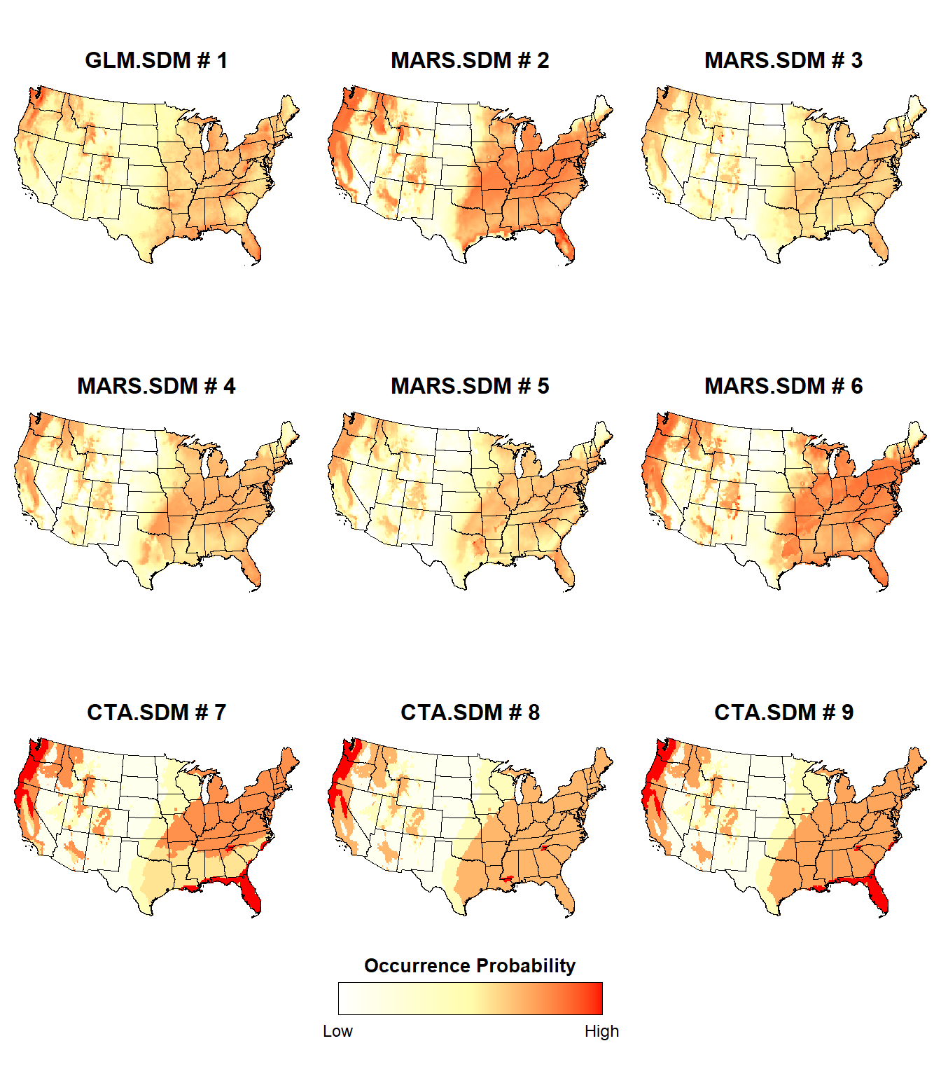
The probability of presence is slightly different between the individual SDMs, although some regions consistently exhibit a high probability of presence (e.g., Pacific Northwest, Ohio River Valley) or a low probability of presence (e.g., the Great Plains)
Now, let’s plot the probability of presence for the individual RF SDMs.
# Last 10 plots (all RF models)
plotList <- lapply(10:19, function(x) {
  d <- stars::st_as_stars(ESDM@sdms[[x]]@projection)
  i = x - 9
  plotFunction(
    d, main_title = paste(ESDM@sdms[[x]]@name, '#', i), cap = NULL, title_size = 12
  )
})
place_plots(p = plotList, legend_position = c(0.6, 2))
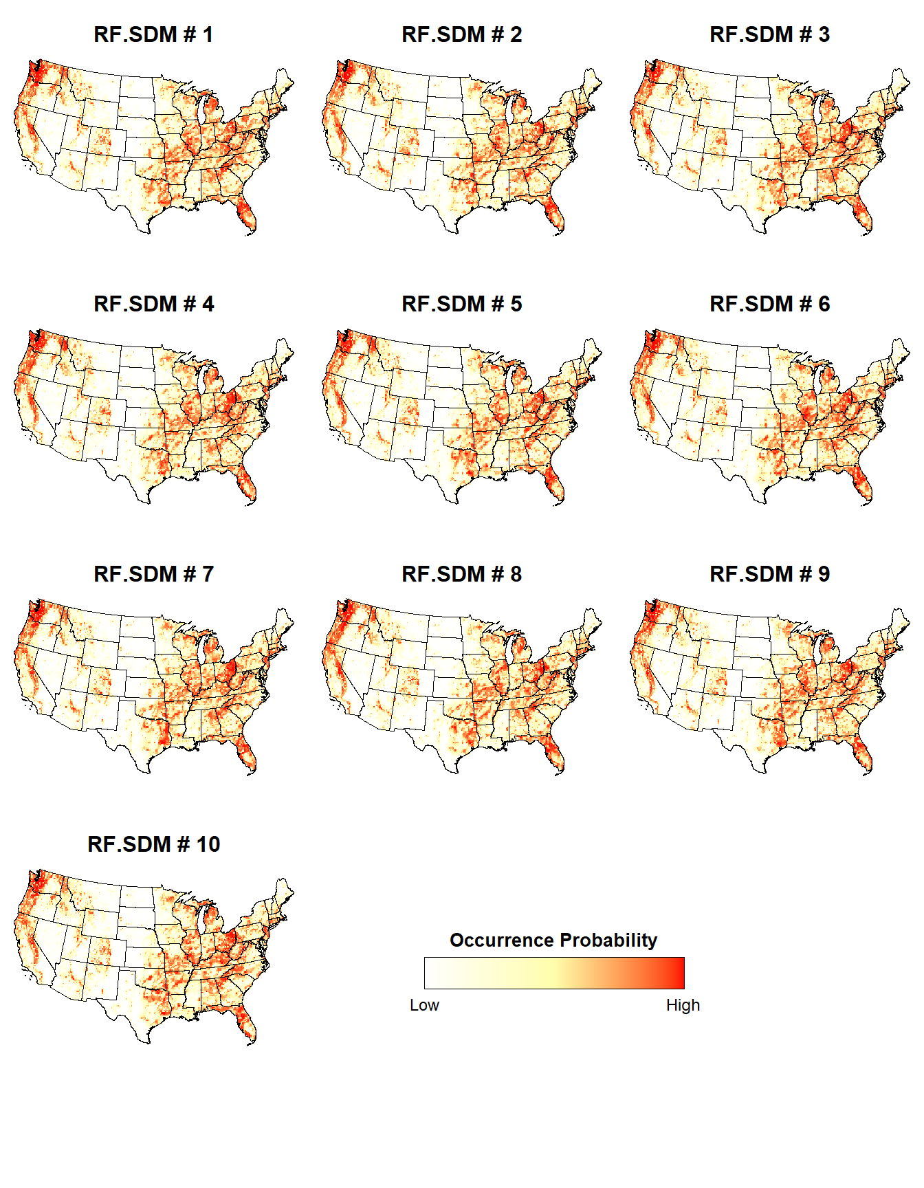
The individual RF SDMs seem to exhibit a relatively consistent probability of presence.
RF SDM
Let’s plot the probability of presence for one of the RF SDMs.
# Plot RF species distribution model within lower 48 states
plotFunction(
  x = stars::st_as_stars(ESDM@sdms[[10]]@projection),
  main_title = 'Probability of Bigfoot Occurrence (RF SDM)',
  cap = 'Data: Bigfoot Field Researchers Organization (bfro.net)',
  title_size = 18, margin = TRUE
)
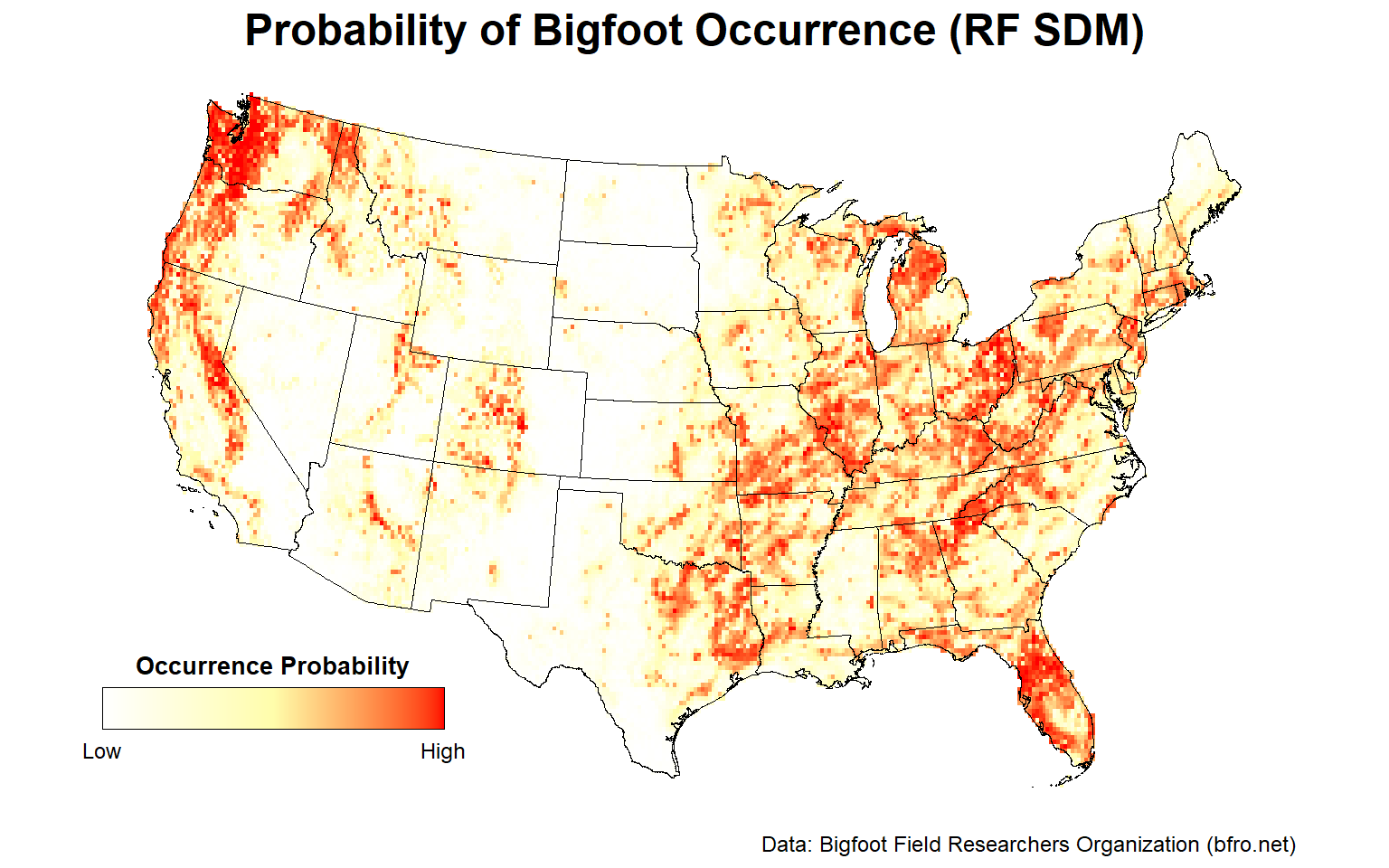
Looking at this map, there are areas that stand out as having a high probability of Bigfoot occurrence. These include the Pacific Northwest, the Ohio River Valley, central Florida, and to a lesser extent, the Sierra Nevada mountain range.
Let’s plot the binary presence/absence map for one of the RF SDMs.
# Plot RF presence/absence binary map
plotFunction(
  x = stars::st_as_stars(ESDM@sdms[[10]]@binary),
  main_title = 'Bigfoot Presence/Absence Binary Map (RF SDM)',
  cap = 'Data: Bigfoot Field Researchers Organization (bfro.net)',
  title_size = 18, margin = TRUE, legend = FALSE
)
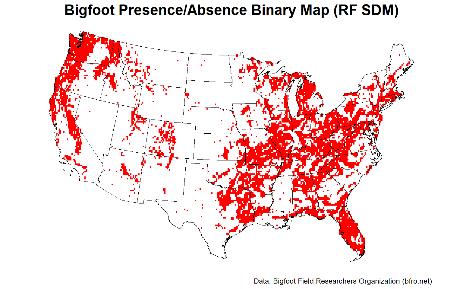
The Pacific Northwest, the Ohio River Valley, and central Florida appear to provide the best habitat for Bigfoot.
Let’s plot variable importance for one of the RF SDMs.
ESDM@sdms[[10]]@variable.importance %>%
  tidyr::gather(Variable, Value) %>%
  mutate(Variable = forcats::fct_reorder(Variable, Value)) %>%
  ggplot(aes(x = Variable, y = Value)) +
  geom_col(fill = '#82B2C3') +
  coord_flip() +
  geom_text(aes(label = round(Value, 2), y = Value + 0.18),
            size = 3, vjust = 1) +
  labs(title = 'Variable Importance',
       subtitle = 'RF Species Distribution Model') +
  theme_classic(base_size = 12) +
  theme(plot.title = element_text(size = 14, hjust = 0,
                        margin = margin(b = 2), face = 'bold'),
        plot.subtitle = element_text(size = 12, hjust = 0,
                          margin = margin(b = 5), face = 'italic'),
        axis.text = element_text(color = 'black'))
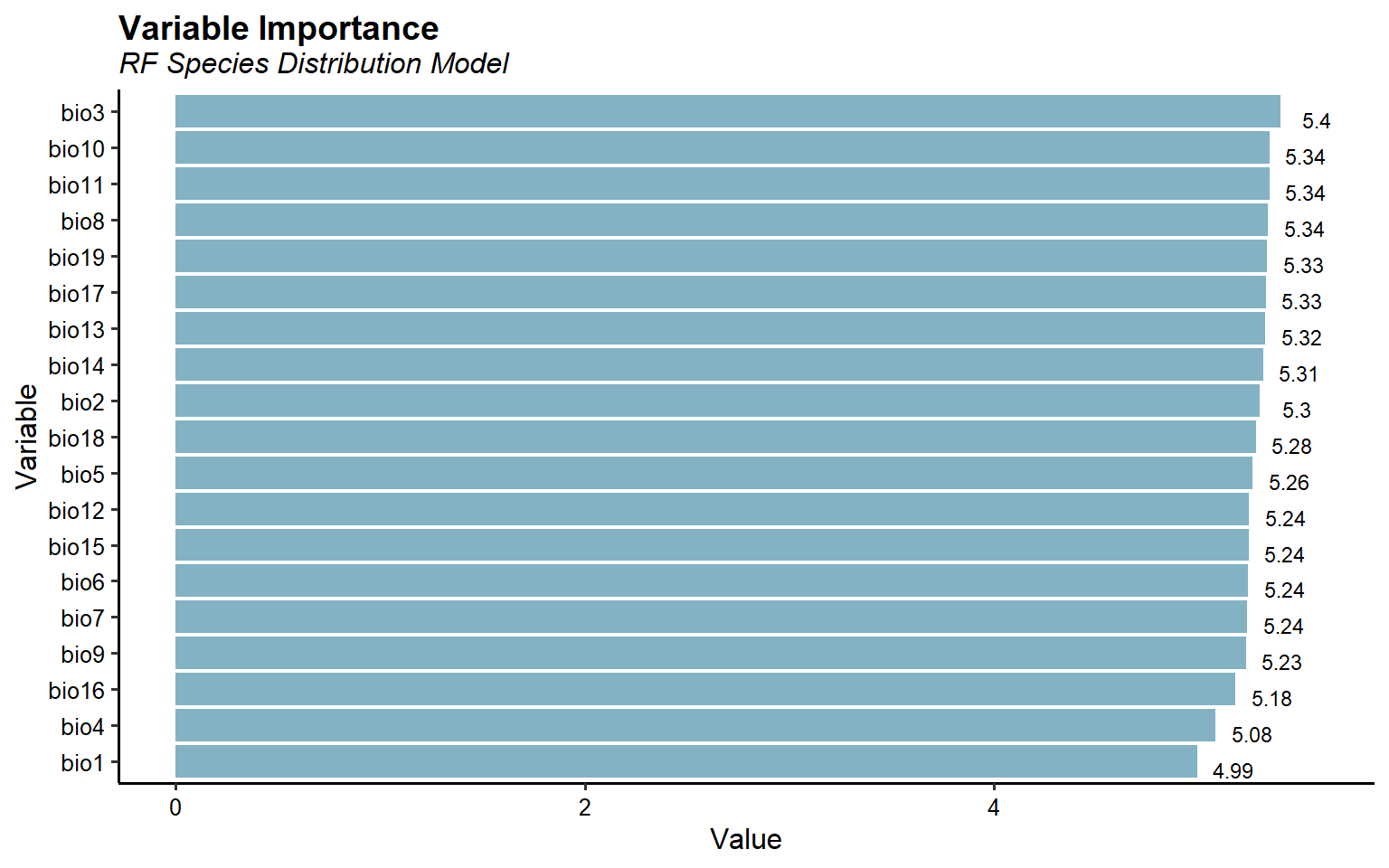
This plots suggest all 19 bioclimatic variables are important for predicting Bigfoot habitat suitability.
Let’s inspect model performance for one of the RF SDMs.
library(kableExtra)
ESDM@sdms[[10]]@evaluation %>%
  mutate_if(is.numeric, round, 3) %>%
  kbl() %>%
  kable_paper(full_width = F, position = 'left')
| threshold | AUC | omission.rate | sensitivity | specificity | prop.correct | Kappa |
|---|---|---|---|---|---|---|
| 0.535 | 0.735 | 0.265 | 0.735 | 0.735 | 0.735 | 0.471 |
Final Ensemble SDM
Let’s plot the probability of presence for the final ensemble SDM comprised of all 19 individual SDAs.
# Plot ensemble species distribution model within lower 48 states
plotFunction(
  x = ESDM_stars,
  main_title = 'Probability of Bigfoot Occurrence (Ensemble SDM)',
  cap = 'Data: Bigfoot Field Researchers Organization (bfro.net)',
  title_size = 18, margin = TRUE
)
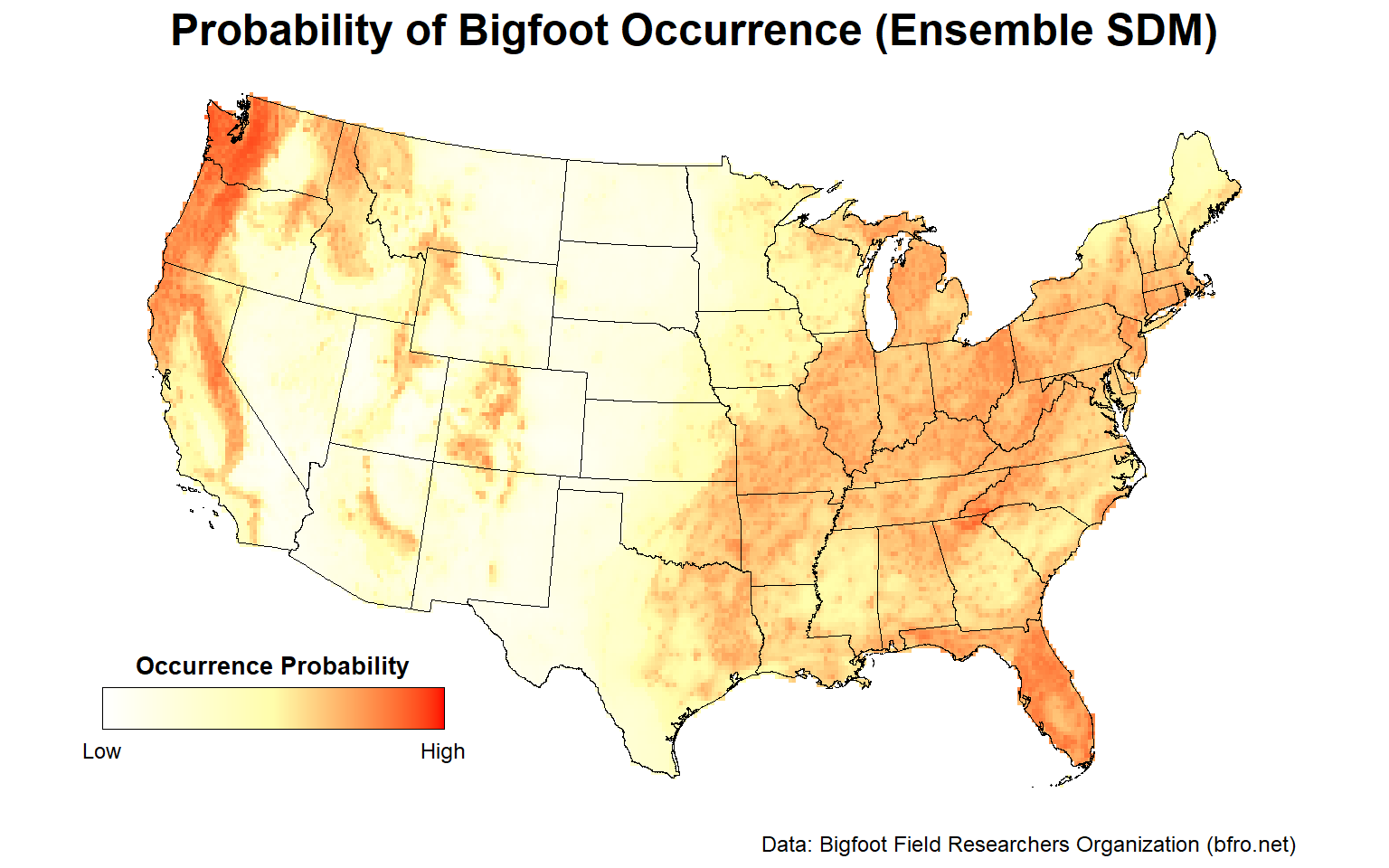
Similar to the individual RF SDM, the Pacific Northwest, the Ohio River Valley, central Florida, and to a lesser extent, the Sierra Nevada mountain range are areas with a high probability of Bigfoot occurrence.
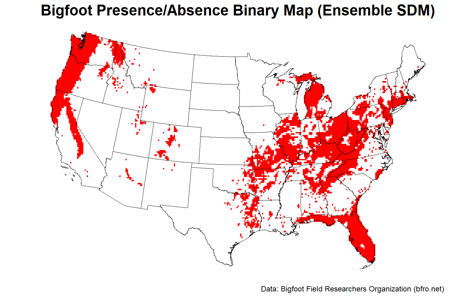
Let’s plot the binary presence/absence map for the final ensemble SDM.
# Plot ensemble presence/absence binary map
plotFunction(
  x = stars::st_as_stars(ESDM@binary),
  main_title = 'Bigfoot Presence/Absence Binary Map (Ensemble SDM)',
  cap = 'Data: Bigfoot Field Researchers Organization (bfro.net)',
  title_size = 18, margin = TRUE, legend = FALSE
)
Let’s plot the uncertainty map for the final ensemble SDM.
# Plot ensemble uncertainty map representing the between-methods variance
plotFunction(
  x = stars::st_as_stars(ESDM@uncertainty),
  main_title = 'SDM Uncertainty Map (Ensemble SDM)',
  cap = 'Uncertainty based on between-methods variance',
  title_size = 18, margin = TRUE,
  type = 'xx', legend = TRUE, maxx = 0.15
)
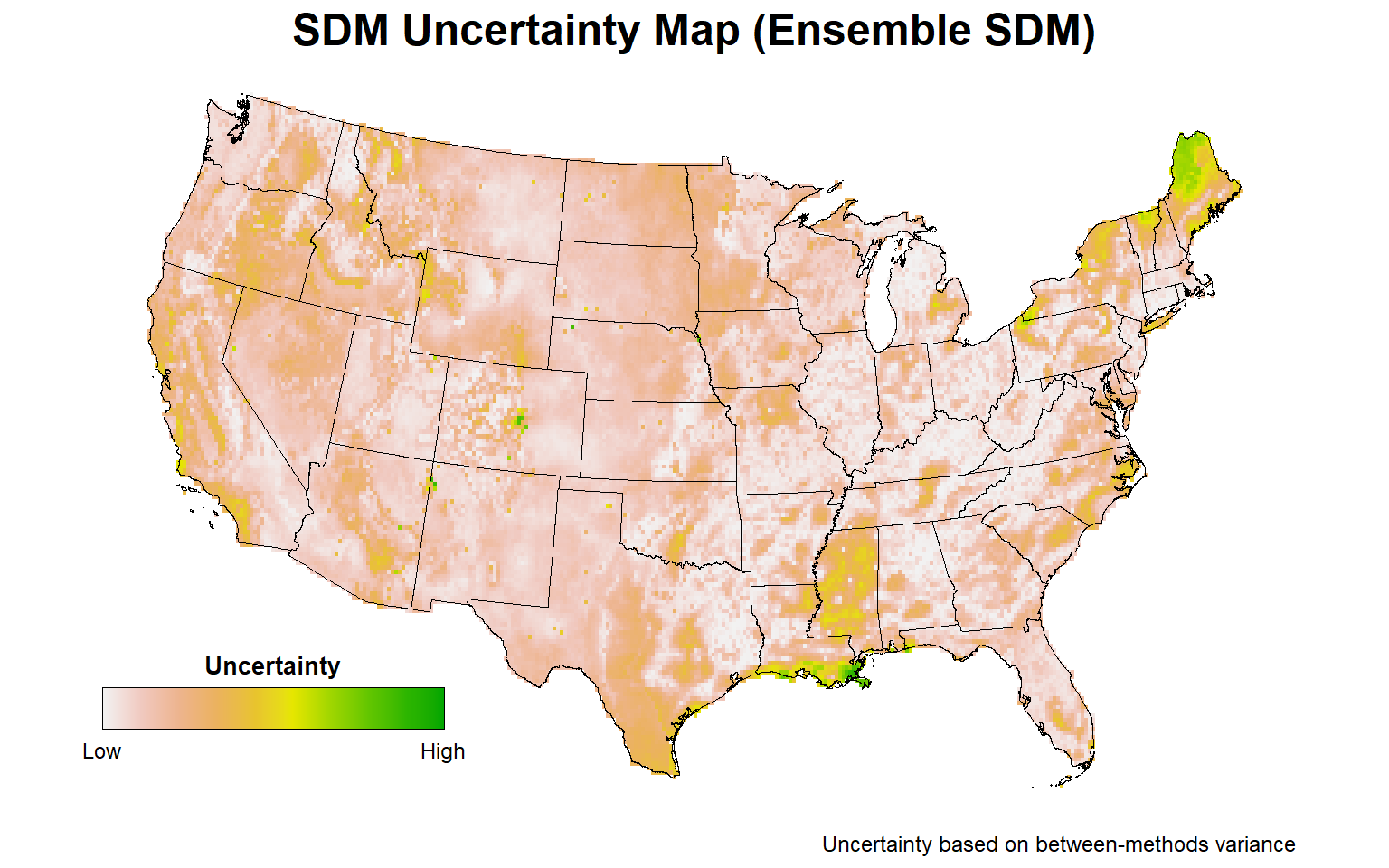
For those areas with a high probability of Bigfoot occurrence, the highest uncertainty is associated with parts of central Florida, particularly the Everglades, the Sierra Nevada mountain range, and parts of the Ohio River Valley. Less uncertainty in predicting Bigfoot occurrence is associated with the Pacific Northwest.
Let’s plot variable importance for the final ensemble SDM.
# Variable importance
ESDM@variable.importance %>%
  tidyr::gather(Variable, Value) %>%
  mutate(Variable = forcats::fct_reorder(Variable, Value)) %>%
  ggplot(aes(x = Variable, y = Value)) +
  geom_col(fill = '#82B2C3') +
  coord_flip() +
  geom_text(aes(label = round(Value, 2), y = Value + 1),
            size = 3, vjust = 1) +
  labs(title = 'Variable Importance',
       subtitle = 'Ensemble Species Distribution Model') +
  theme_classic(base_size = 12) +
  theme(plot.title = element_text(size = 14, hjust = 0,
                        margin = margin(b = 2), face = 'bold'),
        plot.subtitle = element_text(size = 12, hjust = 0,
                          margin = margin(b = 5), face = 'italic'),
        axis.text = element_text(color = 'black'))
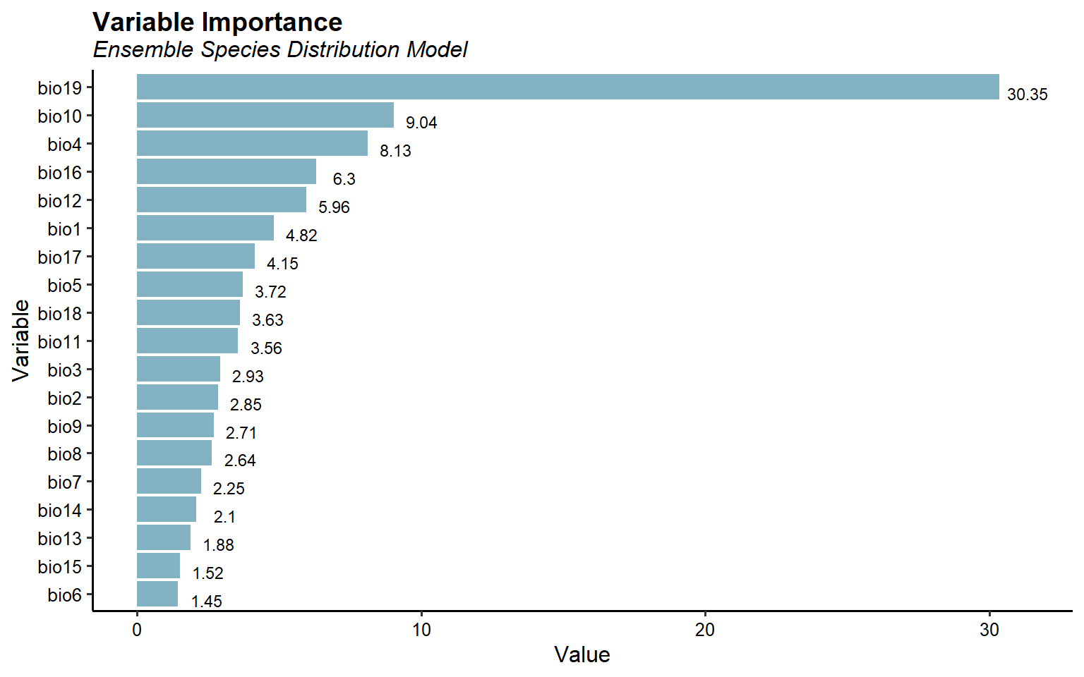
This plots suggest that precipitation of the coldest quarter (bio19) is the most important variable for predicting Bigfoot habitat suitability. Mean temperature of the warmest quarter (bio10) and temperature seasonality (bio4) are the next important variables.
Let’s inspect the model performance for the final ensemble SDM.
ESDM@evaluation %>%
  mutate_if(is.numeric, round, 3) %>%
  kbl() %>%
  kable_paper(full_width = F, position = 'left')
| threshold | AUC | omission.rate | sensitivity | specificity | prop.correct | Kappa |
|---|---|---|---|---|---|---|
| 0.661 | 0.715 | 0.247 | 0.753 | 0.677 | 0.715 | 0.377 |
Final Thoughts
With the development of advanced statistical modelling and the availability of publicly available biodiversity databases, there has been a rapid increase in the use of species distribution modelling. Although SDMs are extremely useful tools, they should be used judiciously. The difficulties come largely from the limits of data. The number of presence observations is often small compared to the number of influential predictors, resulting in a critical problem of over-fitting during modelling. SDMs assume that species are at equilibrium with the environment and that the model has incorporated all major factors determining species range limits. By ignoring global change in the environmental drivers when making transfers to other time periods or geographic areas, considerably bias may be introduced to the resultant predictions.
Another potential source of error that may affect the accuracy of these models is incorrect (or incomplete) taxonomy. This issue may be particularly problematic, for example, with cryptic species or subspecies that are morphologically similar but may have very distinct ecological requirements and geographic distributions, or for those data sources that contain indirect observations rather than references only to physical specimens. For example, Lozier et al. (2009) compared the niche model for Bigfoot to one they developed for the (far less frequently observed) black bear. The two were statistically indistinguishable. This leads one to wonder if many Bigfoot sightings are, in fact, of black bears. However, for those interested in finding Bigfoot, a good place to start is the Pacific Northwest.
References
Brown, J.H. and M.V. Lomolino. 1998. Biogeography. Sinauer Associates, Sunderland, MA.
Elith, J. and J.R. Leathwick. 2009. Species distribution models: ecological explanation and prediction across space and time. Annual Review of Ecology, Evolution, and Systematics. 40, 677-697.
Franklin, J. 2010. Mapping Species Distributions: Spatial Inference and Prediction. Cambridge University Press, Cambridge.
Hijmans, R.J. and J. Elith. 2017. Species Distribution Modeling in R. January.
Hijmans, R.J., S.E. Cameron, J.L. Parra, P. Jones, and A. Jarvis. 2005. Very high resolution interpolated climate surfaces for global land areas. International Journal of Climatology, 25, 1965-1978.
Gaston, K.J. 2003. The Structure and Dynamics of Geographic Ranges. Oxford University Press,Oxford.
Lozier, J.D., P. Aniello, and M.J. Hickerson. 2009. Predicting the distribution of Sasquatch in western North America: anything goes with ecological niche modelling. Journal of Biogeography. 26, 1623-1627.
Meldrum, J. 2007. Sasquatch: Legend Meets Science. Forge Books, NY.
Peterson, A.T., J. Soberon, R.G. Pearson, R.P Anderson, E. Martinez-Meyer, M. Nakamura, and M.B. Araujo. 2011. Ecological Niches and Geographic Distributions. Princeton University Press, Princeton, NJ.
Udvardy, M.D.F. 1969. Dynamic Zoogeography. Van Nostrand Reinhold Company,New York, NY.
Zurell, D. 2020. Introduction to Species Distribution Modelling (SDM) in R. https://damariszurell.github.io/SDM-Intro/.
- Posted on:
- October 12, 2022
- Length:
- 20 minute read, 4109 words
- See Also: