Introduction

Statistical confidence limits are used for addressing uncertainties when calculating the mean concentration from an unknown population. In some circumstances, it makes more sense to express the confidence interval in only one direction - with only a lower confidence limit, or only an upper confidence limit, but not both. For a “one-sided” confidence limit, all the possibility of error is assigned to one side. One-sided confidence limits are essentially an open-ended version of two-sided intervals. The 95% upper confidence limit (95% UCL or UCL95) is often used as an acceptable estimate of the true mean concentration for a sample population. This means there is a 95% chance that the true distribution of the sample data has a population mean less than or equal to the calculated UCL. The UCL95 is used in several environmental applications, including the estimation of contaminant exposure point concentrations for risk assessment purposes and determining the attainment of cleanup standards or other environmental management decisions.

This post presents methods that can be used to calculate a UCL95 on the mean of an unknown population, where all measurements are detections. If the data contain a mixture of detects and non-detects, statistical methods for dealing with censored data should be used. The estimation methods as described in this post are applicable to data sets coming from a single statistical population. The sampled data should represent a random sample from the investigative area such that the data are representative of the entire population under study.

Load Libraries

We’ll start by loading the required R libraries. The main R library that we will be using for the computations is the EnvStats library. EnvStats includes methods for the graphical and statistical analyses of environmental data, with a focus on analyzing chemical concentrations and physical parameters, usually in the context of mandated environmental monitoring.

# Load libraries
library(dplyr)
library(EnvStats)

Data

Let’s load the data and compute descriptive statistics. The data are comprised of arsenic concentrations in 54 surface soil samples. Concentrations range from 2.7 to 32 milligrams-per kilogram (mg/kg) with an average concentration of 9.18 mg/kg and a median concentration of 8.15 mg/kg. The standard deviation is 5.1 mg/kg and the cofficient of variation (CV) is 0.56.

# Read data in comma-delimited file
dat <- read.csv('./data/Arsenic.csv', header = T)

# Assign results to variable Arsenic
Arsenic <- dat$Result

summarytools::descr(Arsenic)
## Descriptive Statistics  
## Arsenic  
## N: 54  
## 
##                     Arsenic
## ----------------- ---------
##              Mean      9.18
##           Std.Dev      5.10
##               Min      2.70
##                Q1      5.60
##            Median      8.15
##                Q3     11.00
##               Max     32.00
##               MAD      4.23
##               IQR      5.35
##                CV      0.56
##          Skewness      1.89
##       SE.Skewness      0.32
##          Kurtosis      5.67
##           N.Valid     54.00
##         Pct.Valid    100.00

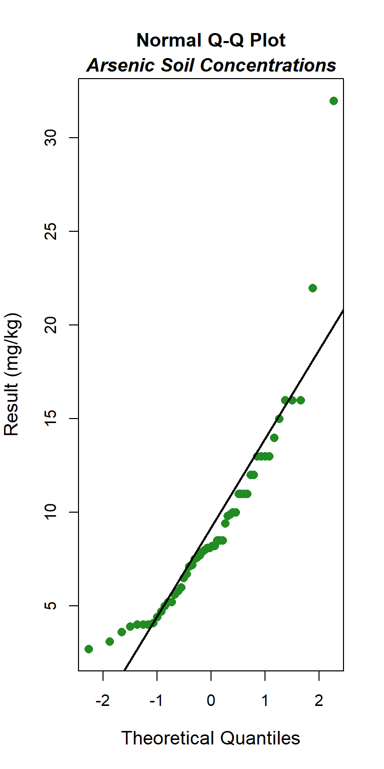
Quantile-quantile (Q-Q) plots showing the ordered sample results versus the corresponding quantiles of a normal, lognormal, and gamma data distribution are shown below. Because quantiles are associated with cumulative probabilities, Q-Q plots are also referred to as probability plots. A normal probability plot is used to evaluate the normality of the distribution of a variable (that is, whether, and to what extent, the distribution of the variable follows the normal distribution). If the data are not normally distributed, they will deviate systematically from a straight line. Variability in the data will cause the data to scatter randomly around this line but the data will still appear to follow a single straight line. In addition to providing information about the data distributions, Q-Q plots are useful in identifying outliers potentially present in a data set. On a Q-Q plot, observations well-separated from the majority of the data may represent potential outliers coming from a population different from the main sample population.

### Normal Q-Q Plot
dist <- 'norm'   # norm, lnorm, or gamma
title <- 'Normal Q-Q Plot'
qqPlot(
  x = Arsenic,
  dist = dist,
  pch = 16, cex = 1.2,
  points.col = 'forestgreen',
  add.line = TRUE, line.lwd = 2,
  xlab = 'Theoretical Quantiles',
  ylab = 'Result (mg/kg)',
  font.lab = 1, cex.lab = 1.2, cex.axis = 1.0,
  main = title, cex.main = 1.2
)
mtext('Arsenic Soil Concentrations',
      side = 3, line = 0.2,
      font = 4, cex = 1.2)

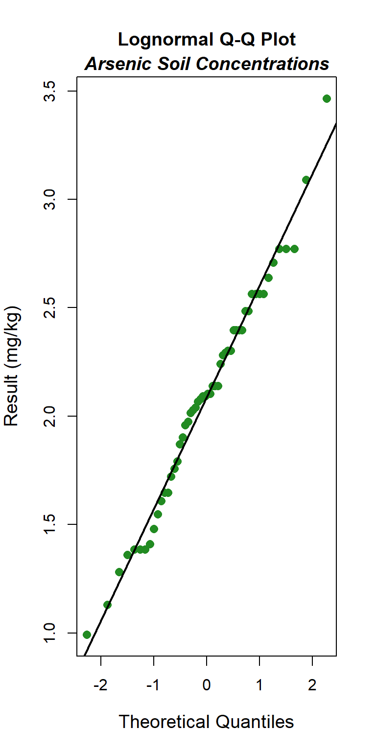
### Logormal Q-Q Plot
dist <- 'lnorm'   # norm, lnorm, or gamma
title <- 'Lognormal Q-Q Plot'
qqPlot(
  x = Arsenic,
  dist = dist,
  pch = 16, cex = 1.2,
  points.col = 'forestgreen',
  add.line = TRUE, line.lwd = 2,
  xlab = 'Theoretical Quantiles',
  ylab = 'Result (mg/kg)',
  font.lab = 1, cex.lab = 1.2, cex.axis = 1.0,
  main = title, cex.main = 1.2
)
mtext('Arsenic Soil Concentrations',
      side = 3, line = 0.2,
      font = 4, cex = 1.2)

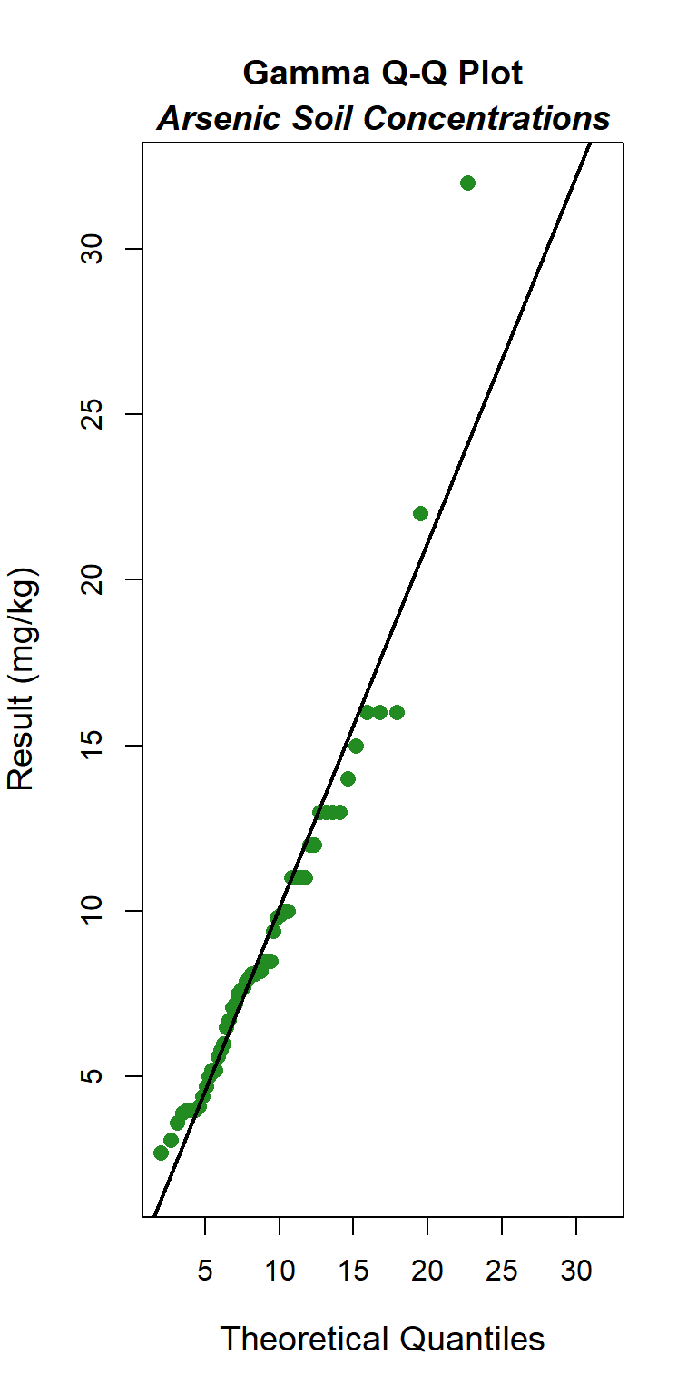
### Gamma Q-Q Plot
dist <- 'gamma'   # norm, lnorm, or gamma
title <- 'Gamma Q-Q Plot'
qqPlot(
  x = Arsenic,
  dist = dist,
  estimate.params = TRUE,
  pch = 16, cex = 1.2,
  points.col = 'forestgreen',
  add.line = TRUE, line.lwd = 2,
  xlab = 'Theoretical Quantiles',
  ylab = 'Result (mg/kg)',
  font.lab = 1, cex.lab = 1.2, cex.axis = 1.0,
  main = title, cex.main = 1.2
)
mtext('Arsenic Soil Concentrations',
      side = 3, line = 0.2,
      font = 4, cex = 1.2)

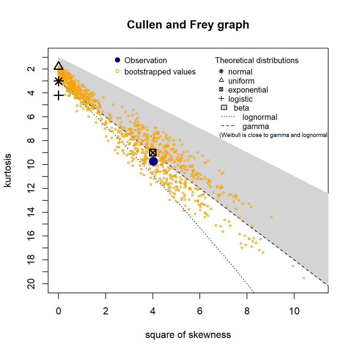
A skewness-kurtosis plot for the empirical distribution of the arsenic concentration data is shown below. On this plot, values for common distributions are displayed to help identify possible distributions to fit to data. For some distributions (e.g., normal), there is only one possible value for the skewness and the kurtosis and the distribution is thus represented by a point on the plot. For other distributions (e.g., lognormal and gamma), areas of possible values are represented by lines. To account for uncertainty in the estimated values of kurtosis and skewness from the data, the values were bootstrapped 1,000 times.

The skewness-kurtosis plot indicates that the data may fit a lognormal or gamma distribution. The Q-Q plots also suggest that the data are lognormally or gamma distributed.

# Load libraries
library(fitdistrplus)

# Use the function descdist to obtain possible candidate distributions
descdist(Arsenic, boot = 1000)
## summary statistics
## ------
## min:  2.7   max:  32 
## median:  8.15 
## mean:  9.17963 
## estimated sd:  5.102769 
## estimated skewness:  2.004597 
## estimated kurtosis:  9.714515

Goodness-of-fit Test

Sample distribution assumptions are important in determining how upper confidence limits for a data set are calculated. Shapiro-Wilk goodness-of-fit (GOF) tests were performed to determine the probability that the arsenic concentration data could have come from the tested distributions. The Shapiro-Wilk test is one of the most commonly used GOF tests for normality.

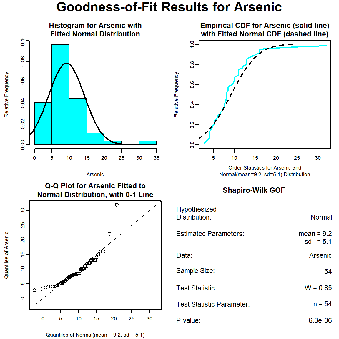
The GOF test assuming a normal distribution is provided below. The p-value is <0.001, indicating that the data are not normally distributed. This also is evident by the curvature of the data in the normal Q-Q plot.

# Run goodness-of-fit test for normal distribution
dat_norm <- gofTest(Arsenic)
plot(dat_norm)

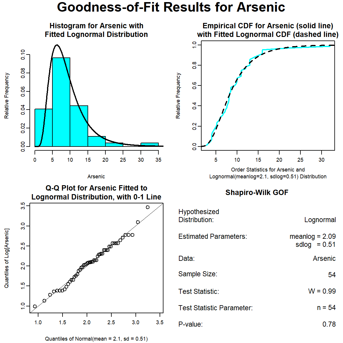
The GOF test assuming a lognormal distribution is provided below. The p-vaue is 0.78, indicating that the data can be assumed to follow a lognormal distribution. This also is evident by visual inspection of the Q-Q plot.

# Run goodness-of-fit test for lognormal distribution
dat_lnorm <- gofTest(Arsenic, dist = "lnorm")
plot(dat_lnorm)

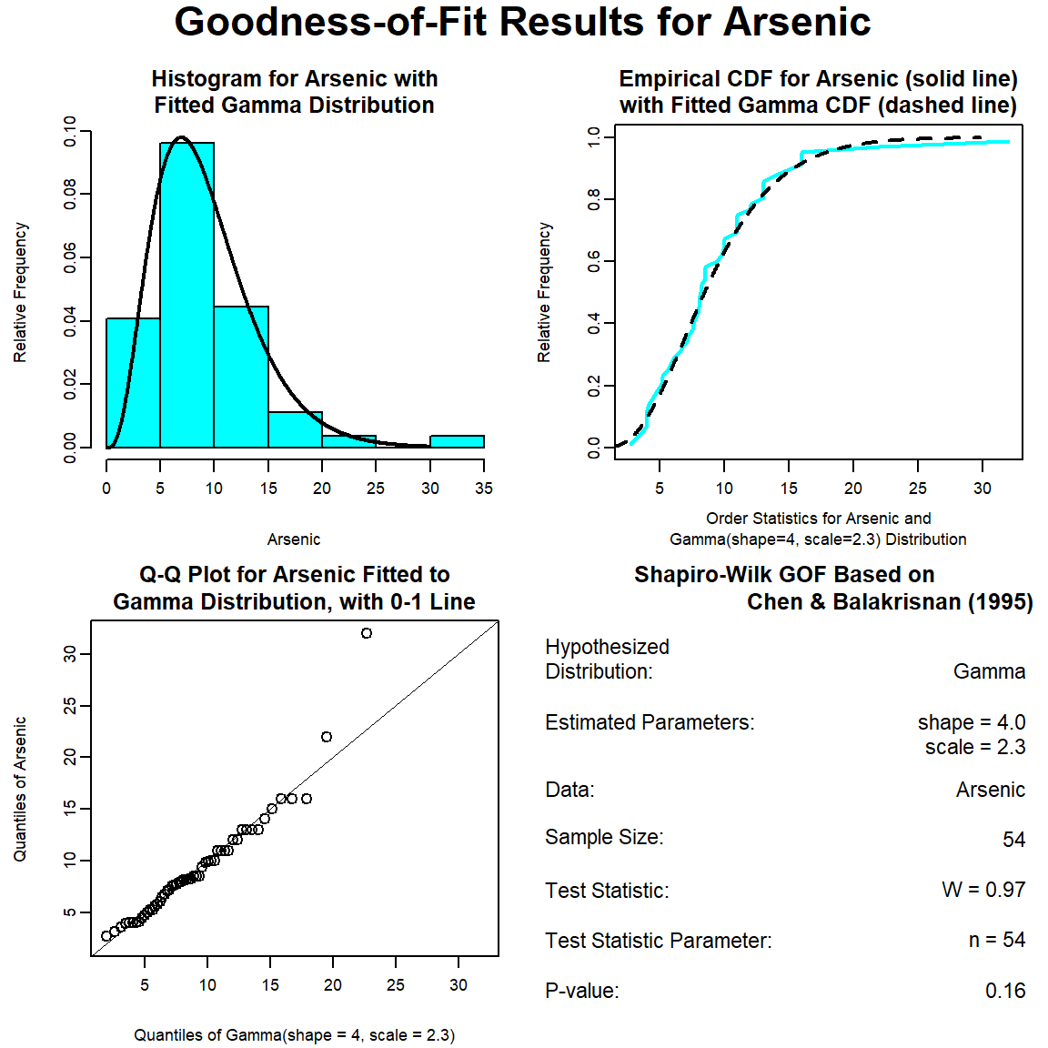
The GOF test assuming a gamma distribution is provided below. The p-vaue is 0.16, indicating that the data can be assumed to follow a gamma distribution. This also is evident by visual inspection of the Q-Q plot, although the maximum concentration appears far removed from the theoretical distribution.

# Run goodness-of-fit test for gamma distribution
dat_gamma <- gofTest(Arsenic, dist = "gamma")
plot(dat_gamma)

Various GOF statistics were computed for the three distributions (normal, lognormal, and gamma) tested and the results are provided below. The GOF statistics measure the distance between the fitted parametric distribution and the empirical distribution. All the GOF statistics favor the lognormal distribution. The difference in values of the test statistics between the lognormal and gamma distributions is relatively minor and thus, the choice between these two distributions could be discussed.

# Fit a few possible distributions
fn <- fitdist(Arsenic, "norm")
fln <- fitdist(Arsenic, "lnorm")
fg <- fitdist(Arsenic, "gamma")

# Compute different goodness-of-fit statistics
gofstat(
 list(fn, fln, fg),
 fitnames = c("normal", "lognormal", "gamma")
)
## Goodness-of-fit statistics
##                                 normal  lognormal      gamma
## Kolmogorov-Smirnov statistic 0.1460649 0.07197230 0.08658389
## Cramer-von Mises statistic   0.2163225 0.04454104 0.04098636
## Anderson-Darling statistic   1.4824246 0.29199546 0.32926514
## 
## Goodness-of-fit criteria
##                                  normal lognormal    gamma
## Akaike's Information Criterion 332.2526  308.9634 311.8109
## Bayesian Information Criterion 336.2306  312.9413 315.7889

Upper Confidence Limit

Various methods were used to calcuate the UCL95 of the mean arsenic concentration for the sample population and the results are shown below. Methods that were used include the Student’s t-UCL, lognormal UCL based on Land’s H-statistic, gamma UCL, and percentile bootstrap UCL. The percentile bootstrap UCL is a nonparametric method that does not rely on a distributional assumption.

### Normal UCL95
# Options include "mvue"(minimum  variance  unbiased) and "mle/mme" (maximum
# likelihood/method of moments).
ucl_norm <- enorm(
  x = Arsenic,
  method = "mvue",
  ci = TRUE,
  ci.type = "upper",
  ci.method = "exact",
  conf.level = 0.95,
  ci.param = "mean"
)

### Gamma UCL95
# Options include "kulkarni.powar", "cube.root", and "fourth.root".
ucl_gamma <- egammaAlt(
  x = Arsenic,
  method = "bcmle",
  ci = TRUE,
  ci.type = "upper",
  ci.method = "normal.approx",
  normal.approx.transform = "kulkarni.powar",
  conf.level = 0.95
)

### Lognormal UCL95 Land H-Statistic
# Options include "land" (Land?s method; the default), zou (Zou et al. method),
# "parkin" (Parkin et al. method), "cox" (Cox?s approximation), and
# "normal.approx" (normal approximation).
ucl_lnormAlt <- elnormAlt(
  x = Arsenic,
  method = "mvue",
  ci = TRUE,
  ci.type = "upper",
  ci.method = "land",
  conf.level = 0.95,
  parkin.list = NULL
)

### Bootstap UCL95
# Load library
library(boot)

# Set seed
set.seed(123)

# Create function to compute mean
samplemean <- function(x, d) {
  return(mean(x[d]))
}

# Run bootstrap and get confidence interval
bootmean <- boot(Arsenic, statistic = samplemean, R = 10000)
ucl_bs <- boot.ci(bootmean, conf = 0.90, type = "perc")

For this data set, the results are remarkably similar. The UCL95 of the mean arsenic concentration ranges from 10.3 mg/kg, assuming either a normal or gamma distribution, to 10.5 mg/kg for a lognormal distribution. The nonparametric percentile bootstrap UCL95 is 10.4 mg/kg. Because the data do not conform to a normal distribution, final selection of the UCL95 should consider one of the other computational methods.

### Compare results
data.frame(
  normal = ucl_norm$interval$limits[[2]],
  lognormal = ucl_lnormAlt$interval$limits[[2]],
  gamma = ucl_gamma$interval$limits[[2]],
  bootstrap = ucl_bs$perc[[5]]
) %>% round(2)
##   normal lognormal gamma bootstrap
## 1  10.34     10.48 10.33     10.37

As a note, environmental data are frequently right-skewed, and right-skewed data often follow a lognormal distribution. However, use of a parametric lognormal distribution on a lognormally distributed data set may yield unrealistically large upper limits, especially when the standard deviation of the log-transformed data becomes greater than 1 for small data sets (less than 30 to 50 measurements). Because environmental data typically can be modeled by a gamma distribution, gamma distribution limits generally are given preference over lognormal distribution limits, where appropriate.