Generalized Least Squares Regression

By Charles Holbert

April 17, 2024

Introduction

The estimation of and inference from ordinary least squares (OLS) regression depend on several assumptions. One assumption is that the errors are independent and identically distributed. Unequal variances of residuals, referred to as heteroskedasticity, can lead to biased estimators and incorrect standard errors. It is important to diagnose and address heteroskedasticity in regression analysis to ensure the validity and reliability of the results. This can be done through visual inspection of residuals as well as formal statistical tests. Alternative methods like generalized least squares (GLS) and weighted least squares (WLS) regression can be considered when OLS assumptions are violated. GLS is used for dependent errors, while WLS is used for independent but non-identically distributed errors. WLS is a special case of GLS, in that the error terms for each observation may have its own variance, but are pairwise independent.

In this blog post, we will explore methods to identify heteroscedasticity and work through an example to address non-constant variance and correlated standard errors using GLS and WLS regression. The analyses will be conducted using the R language for statistical computing and visualization.

Data

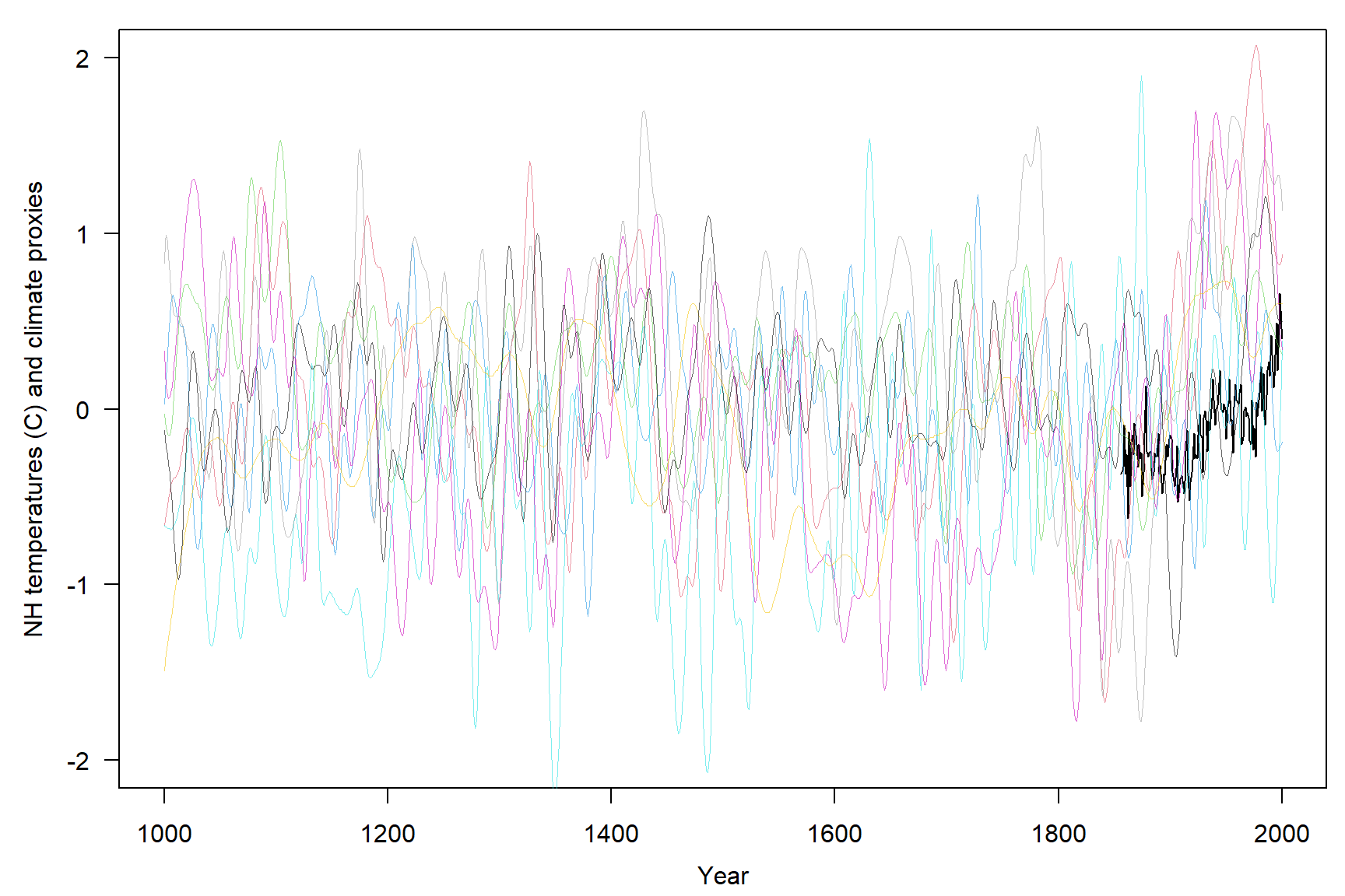
The data used in this example is the globwarm dataset that is contained in the faraway package. The globwarm dataset contains average Northen Hemisphere Temperatures from 1856 through 2000 and eight climate proxies from 1000 to 2000AD. Reliable records of temperature are only available back to the 1850s. Proxy measures of temperature are available that go back much longer. For example, trees grow faster in warmer years so the width of tree rings (seen in tree crosssections) provides some evidence of past temperatures. Other natural sources of climate proxies include coral and ice cores. Such information can go back for a thousand years or more.

The globwarm dataset contains 1,001 observations on the following 10 variables:

nhtemp: Northern hemisphere average temperature (C) provided by the UK Met Office
wusa: Tree ring proxy information from the Western USA
jasper: Tree ring proxy information from Canada
westgreen: Ice core proxy information from west Greenland
chesapeake: Sea shell proxy information from Chesapeake Bay
tornetrask: Tree ring proxy information from Sweden
urals: Tree ring proxy information from the Urals
mongolia: Tree ring proxy information from Mongolia
tasman: Tree ring proxy information from Tasmania
year: Year 1000-2000AD

# Load libraries
library(dplyr)
library(faraway)
library(ggplot2)
library(scales)

# Load plotting function
source('functions/plot_functions.R')

# Read data in comma-delimited file
data(globwarm)

# Inspect data
str(globwarm)
## 'data.frame':	1001 obs. of  10 variables:
##  $ nhtemp    : num  NA NA NA NA NA NA NA NA NA NA ...
##  $ wusa      : num  -0.66 -0.63 -0.6 -0.55 -0.51 -0.47 -0.43 -0.41 -0.4 -0.39 ...
##  $ jasper    : num  -0.03 -0.07 -0.11 -0.14 -0.15 -0.15 -0.13 -0.07 0 0.09 ...
##  $ westgreen : num  0.03 0.09 0.18 0.3 0.41 0.52 0.6 0.64 0.65 0.63 ...
##  $ chesapeake: num  -0.66 -0.67 -0.67 -0.68 -0.68 -0.68 -0.69 -0.68 -0.67 -0.66 ...
##  $ tornetrask: num  0.33 0.21 0.13 0.08 0.06 0.07 0.09 0.13 0.18 0.25 ...
##  $ urals     : num  -1.49 -1.44 -1.39 -1.34 -1.3 -1.25 -1.2 -1.16 -1.11 -1.07 ...
##  $ mongolia  : num  0.83 0.96 0.99 0.95 0.87 0.77 0.67 0.61 0.56 0.54 ...
##  $ tasman    : num  -0.12 -0.17 -0.22 -0.26 -0.31 -0.37 -0.45 -0.54 -0.64 -0.74 ...
##  $ year      : int  1000 1001 1002 1003 1004 1005 1006 1007 1008 1009 ...

Let’s create a simple plot showing all variables.

par(las = 1, mgp = c(2.4, 1, 0), mar = c(3.6, 4, 1, 0.6))
plot(
  globwarm$year, globwarm$nhtemp,
  type = 'l', lwd = 1, cex.lab = 1,
  ylim = c(-2, 2),
  xlab = 'Year',
  ylab = 'NH temperatures (C) and climate proxies',
)
for(i in 2:9)
  lines(globwarm$year, globwarm[, i], col = alpha(i, 0.6), lwd = 0.5)

Let’s remove missing values so that we have a complete dataset.

dat <- na.omit(globwarm)
rownames(dat) <- seq(length = nrow(dat))

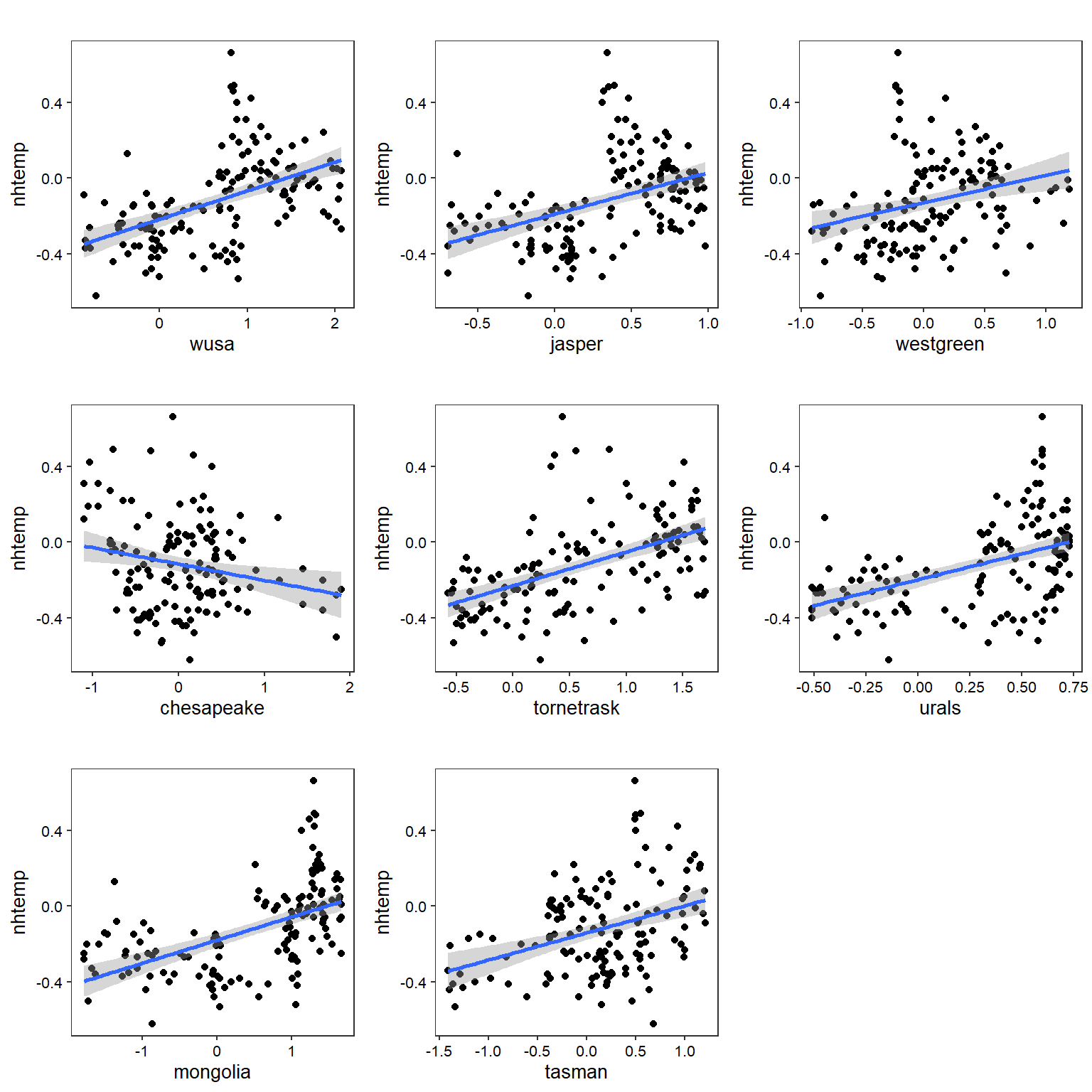
Let’s create individual OLS regression plots for all variables.

# Regression plots of complete data
makeplots <- function(xvar) {
  ggplot(data = dat, aes_(x = as.name(xvar), y = ~nhtemp)) +
    geom_point() +
    stat_smooth(method = 'lm', formula = y ~ x) +
    labs(title = '',
         x = xvar,
         y = 'nhtemp') +
    theme_bw(base_size = 10) +
    theme(panel.grid = element_blank(),
          axis.text = element_text(color = 'black'))
}
vars <- setdiff(colnames(dat), c('nhtemp', 'year'))
plots <- lapply(vars, makeplots)
cowplot::plot_grid(plotlist = plots)

OLS Regression

Let’s fit an OLS regression model with temperature as the response and the eight proxies as predictors. Because we previously removed missing values, the model uses data from 1856 through 2000.

# Linear regression
lmod <- lm(
  nhtemp ~ wusa + jasper + westgreen + chesapeake + tornetrask +
  urals + mongolia + tasman,
  data = dat
)
summary(lmod)
## 
## Call:
## lm(formula = nhtemp ~ wusa + jasper + westgreen + chesapeake + 
##     tornetrask + urals + mongolia + tasman, data = dat)
## 
## Residuals:
##      Min       1Q   Median       3Q      Max 
## -0.43668 -0.11170  0.00698  0.10176  0.65352 
## 
## Coefficients:
##              Estimate Std. Error t value Pr(>|t|)    
## (Intercept) -0.242555   0.027011  -8.980 1.97e-15 ***
## wusa         0.077384   0.042927   1.803 0.073647 .  
## jasper      -0.228795   0.078107  -2.929 0.003986 ** 
## westgreen    0.009584   0.041840   0.229 0.819168    
## chesapeake  -0.032112   0.034052  -0.943 0.347346    
## tornetrask   0.092668   0.045053   2.057 0.041611 *  
## urals        0.185369   0.091428   2.027 0.044567 *  
## mongolia     0.041973   0.045794   0.917 0.360996    
## tasman       0.115453   0.030111   3.834 0.000192 ***
## ---
## Signif. codes:  0 '***' 0.001 '**' 0.01 '*' 0.05 '.' 0.1 ' ' 1
## 
## Residual standard error: 0.1758 on 136 degrees of freedom
## Multiple R-squared:  0.4764,	Adjusted R-squared:  0.4456 
## F-statistic: 15.47 on 8 and 136 DF,  p-value: 5.028e-16

A useful diagnostic of the model is a plot of the residuals against the fitted values. For equal variance (known as homoscedasticity), there should be constant symmetrical variation in the vertical direction. Nonconstant variation in the vertical direction indicates heteroscedasticity.

plot(lmod, 1)
abline(h = 0, col = 'black')

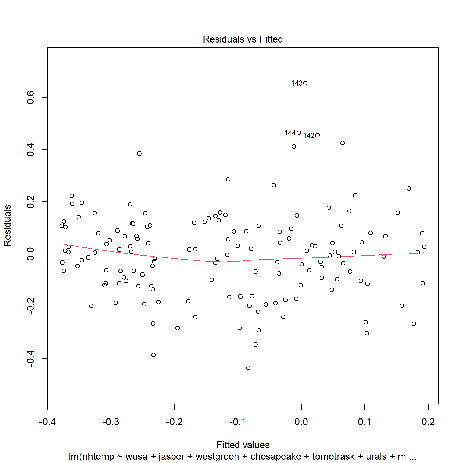
If the errors were uncorrelated, we would expect a random scatter of points above and below the residuals = 0 line. In this plot, we see long sequences of points above or below the line. This is an indication of positive serial correlation.

Let’s see if the residuals are serially correlated by plotting successive pairs of residuals.

n <- length(residuals(lmod))
cor(residuals(lmod)[-1], residuals(lmod)[-n])
## [1] 0.583339

plot(
  tail(residuals(lmod), n-1) ~ head(residuals(lmod), n-1),
  main = 'Diagnostic Plot for Correlated Errors',
  xlab = expression(hat(epsilon)[i]),
  ylab = expression(hat(epsilon)[i+1])
)
abline(h = 0, v = 0, col = 'grey40')

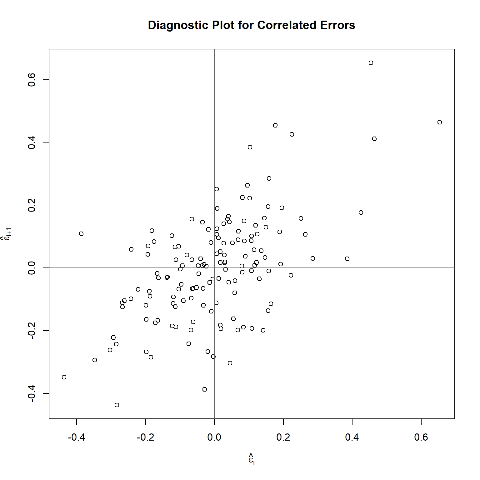
The plot indicates positive serial correlation, which is confirmed by the model shown below. The intercept term is omitted because the residuals have mean zero.

sumary(lm(tail(residuals(lmod), n-1) ~ head(residuals(lmod), n-1)-1))
##                              Estimate Std. Error t value  Pr(>|t|)
## head(residuals(lmod), n - 1) 0.595076   0.069312  8.5855 1.391e-14
## 
## n = 144, p = 1, Residual SE = 0.13918, R-Squared = 0.34

Let’s inspect the residuals using the plot.residuals() function, which produces a time series plot of the residuals, an autocorrelation function (ACF) plot, a partial autocorrelation function (PACF) plot, and performs a Ljung-Box test for residual autocorrelation.

plot.residuals(dat$year, resid(lmod), xlab = 'Year', ylab = 'Residuals')

## 
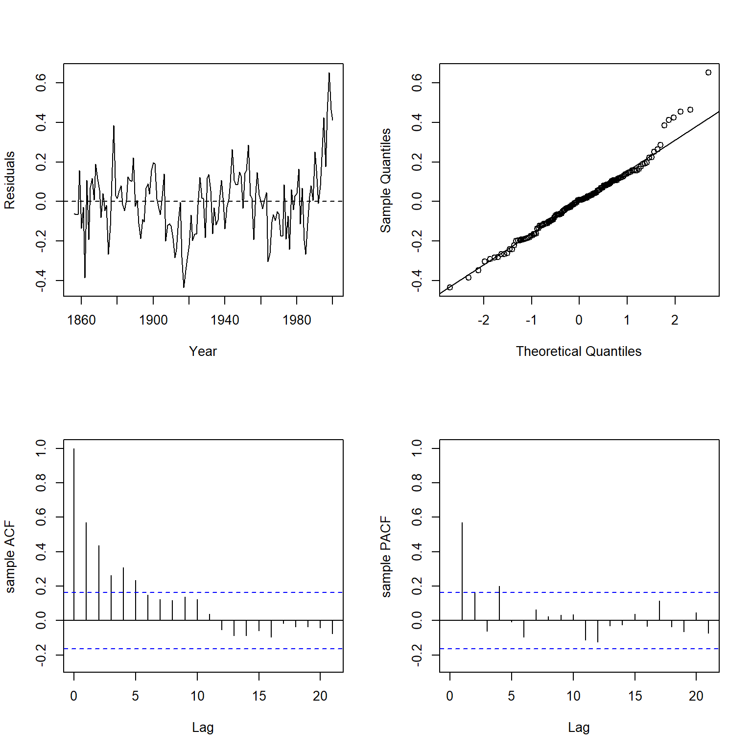
## 	Box-Ljung test
## 
## data:  y
## X-squared = 129.94, df = 21, p-value < 2.2e-16

There is clearly significant positive autocorrelation in the residuals.

A more formal, mathematical way of detecting heteroskedasticity is what is known as the Breusch-Pagan test. The Breusch-Pagan test is an likelihhod ratio test, based on the score of the log likelihood function, calculated under normality. It is a general test designed to detect any linear forms of heteroskedasticity. It tests the null hypothesis that heteroskedasticity is not present (i.e. homoskedastic) against the alternative hypothesis that heteroskedasticity is present. The test is implemented in the lmtest package.

lmtest::bptest(lmod)
## 
## 	studentized Breusch-Pagan test
## 
## data:  lmod
## BP = 45.084, df = 8, p-value = 3.548e-07

Because the p-value from the test is <0.001, we reject the null hypothesis and conclude that heteroscedasticity is a problem in this model.

The Durbin Watson statistic is used as a test for checking autocorrelation in the residuals of a statistical regression analysis. The Durbin-Watson test evaluates errors for first-order autocorrelation where the null hypothesis is that the errors are uncorrelated and the alternative hypothesis is that first-order correlation exists. The test is implemented in the lmtest package.

lmtest::dwtest(
  nhtemp ~ wusa + jasper + westgreen + chesapeake + tornetrask +
  urals + mongolia + tasman,
  data = dat
)
## 
## 	Durbin-Watson test
## 
## data:  nhtemp ~ wusa + jasper + westgreen + chesapeake + tornetrask +     urals + mongolia + tasman
## DW = 0.81661, p-value = 1.402e-15
## alternative hypothesis: true autocorrelation is greater than 0

The p-value from the test indicates strong evidence of serial correlation. It is not surprising to see significant autocorrelation in the data because the proxies can only partially predict the temperature and there is likely some carryover effect from one year to the next.

From the results shown above, we can be confident that there is heteroscedasticity and correlation of errors in the data.

WLS Regression

WLS can be used if the errors are uncorrelated, but the variance of the errors are not the same. WLS regression assigns weights to data points based on variance of fitted values to minimize the sum of weighted squared residuals. Correct weights can replace heteroscedasticity with homoscedasticity. Determining the source of heteroscedasticity may be challenging, so an alternative is estimating variances by using residuals as weights. High variability cases receive low weights, while low variability cases receive high weights.

# Define weights
wts <- 1/lm(abs(lmod$residuals) ~ lmod$fitted.values)$fitted.values^2

# Perform weighted least squares regression
wmod1 <- lm(
  nhtemp ~ wusa + jasper + westgreen + chesapeake + tornetrask +
  urals + mongolia + tasman,
  data = dat,
  weights = wts
)
summary(wmod1)
## 
## Call:
## lm(formula = nhtemp ~ wusa + jasper + westgreen + chesapeake + 
##     tornetrask + urals + mongolia + tasman, data = dat, weights = wts)
## 
## Weighted Residuals:
##     Min      1Q  Median      3Q     Max 
## -3.2099 -0.8718  0.0437  0.7185  4.8637 
## 
## Coefficients:
##              Estimate Std. Error t value Pr(>|t|)    
## (Intercept) -0.245959   0.025213  -9.755  < 2e-16 ***
## wusa         0.088684   0.041447   2.140 0.034163 *  
## jasper      -0.201905   0.078044  -2.587 0.010729 *  
## westgreen    0.008943   0.039649   0.226 0.821895    
## chesapeake  -0.031810   0.035270  -0.902 0.368705    
## tornetrask   0.105839   0.045586   2.322 0.021732 *  
## urals        0.123514   0.083211   1.484 0.140032    
## mongolia     0.038607   0.045111   0.856 0.393598    
## tasman       0.104977   0.027536   3.812 0.000208 ***
## ---
## Signif. codes:  0 '***' 0.001 '**' 0.01 '*' 0.05 '.' 0.1 ' ' 1
## 
## Residual standard error: 1.345 on 136 degrees of freedom
## Multiple R-squared:  0.4735,	Adjusted R-squared:  0.4425 
## F-statistic: 15.29 on 8 and 136 DF,  p-value: 7.275e-16

Let’s inspect the residuals of the WLS model using the plot.residuals() function.

plot.residuals(dat$year, weighted.residuals(wmod1), xlab = 'Year', ylab = 'Residuals')

## 
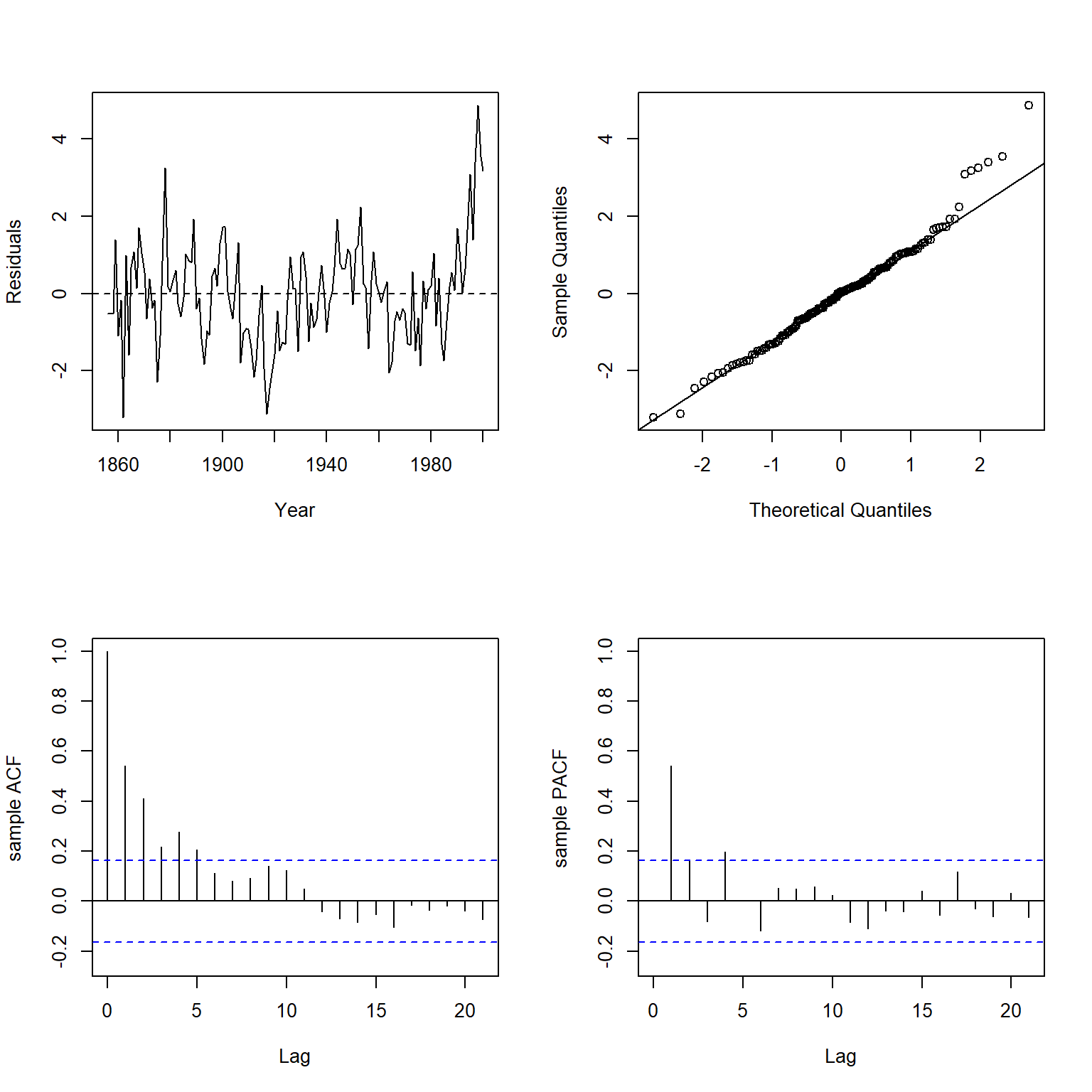
## 	Box-Ljung test
## 
## data:  y
## X-squared = 109.68, df = 21, p-value = 5.385e-14

There is clear evidence of significant positive autocorrelation in the residuals of the model. To remove the autocorrelation from the model, let’s introduce a lag term of the response variable (temperature) to the WLS model.

wmod2 <- lm(
  nhtemp ~ wusa + jasper + westgreen + chesapeake + tornetrask +
  urals + mongolia + tasman + I(lag(nhtemp)),
  data = dat,
  weights = wts
)
summary(wmod2)
## 
## Call:
## lm(formula = nhtemp ~ wusa + jasper + westgreen + chesapeake + 
##     tornetrask + urals + mongolia + tasman + I(lag(nhtemp)), 
##     data = dat, weights = wts)
## 
## Weighted Residuals:
##     Min      1Q  Median      3Q     Max 
## -3.1784 -0.6134  0.0600  0.6432  2.7830 
## 
## Coefficients:
##                 Estimate Std. Error t value Pr(>|t|)    
## (Intercept)    -0.104950   0.027130  -3.868  0.00017 ***
## wusa            0.033345   0.035019   0.952  0.34271    
## jasper         -0.086759   0.066101  -1.313  0.19159    
## westgreen       0.003672   0.032793   0.112  0.91101    
## chesapeake     -0.011378   0.029220  -0.389  0.69760    
## tornetrask      0.047483   0.038309   1.239  0.21734    
## urals           0.058818   0.069552   0.846  0.39925    
## mongolia        0.019258   0.037550   0.513  0.60888    
## tasman          0.051193   0.023708   2.159  0.03261 *  
## I(lag(nhtemp))  0.566916   0.070096   8.088 3.21e-13 ***
## ---
## Signif. codes:  0 '***' 0.001 '**' 0.01 '*' 0.05 '.' 0.1 ' ' 1
## 
## Residual standard error: 1.11 on 134 degrees of freedom
##   (1 observation deleted due to missingness)
## Multiple R-squared:  0.6438,	Adjusted R-squared:  0.6198 
## F-statistic: 26.91 on 9 and 134 DF,  p-value: < 2.2e-16

Let’s inspect the residuals of this new WLS model using the plot.residuals() function.

plot.residuals(
  dat$year[-1], weighted.residuals(wmod2),
  xlab = 'Year', ylab = 'Residuals'
)

## 
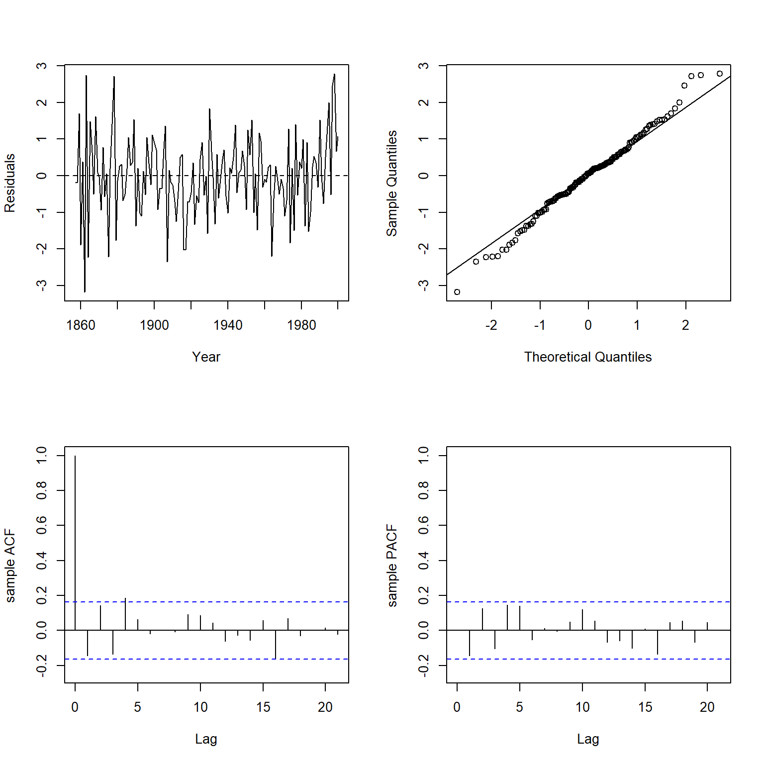
## 	Box-Ljung test
## 
## data:  y
## X-squared = 24.618, df = 21, p-value = 0.2641

The significant positive autocorrelation that was present in the first WLS model is not present in this second WLS model.

GLS Regression

GLS regression extends OLS estimation of the normal linear model by allowing the errors to be correlated and/or have unequal variances. A common application of GLS regression is to time-series analysis, in which it is generally implausible to assume that errors are independent. The gls() function in the nlme package fits regression models with a variety of correlated-error and non-constant error-variance structures. If a correlation or difference of residual variance is not specified within the gls() function, the results are equal to those obtained from the lm() function.

Let’s fit the data using a GLS regression model with a first-order autoregression [AR(1)] error structure.

# Load library
library(nlme)

# Fit GLS with an AR(1) error structure
glmod1 <- gls(
  nhtemp ~ wusa + jasper + westgreen + chesapeake + tornetrask +
  urals + mongolia + tasman,
  correlation = corAR1(form = ~ year),
  data = dat
)
summary(glmod1)
## Generalized least squares fit by REML
##   Model: nhtemp ~ wusa + jasper + westgreen + chesapeake + tornetrask +      urals + mongolia + tasman 
##   Data: dat 
##         AIC       BIC   logLik
##   -108.2074 -76.16822 65.10371
## 
## Correlation Structure: AR(1)
##  Formula: ~year 
##  Parameter estimate(s):
##       Phi 
## 0.7109922 
## 
## Coefficients:
##                   Value  Std.Error   t-value p-value
## (Intercept) -0.23010624 0.06702406 -3.433188  0.0008
## wusa         0.06673819 0.09877211  0.675678  0.5004
## jasper      -0.20244335 0.18802773 -1.076668  0.2835
## westgreen   -0.00440299 0.08985321 -0.049002  0.9610
## chesapeake  -0.00735289 0.07349791 -0.100042  0.9205
## tornetrask   0.03835169 0.09482515  0.404446  0.6865
## urals        0.24142199 0.22871028  1.055580  0.2930
## mongolia     0.05694978 0.10489786  0.542907  0.5881
## tasman       0.12034918 0.07456983  1.613913  0.1089
## 
##  Correlation: 
##            (Intr) wusa   jasper wstgrn chespk trntrs urals  mongol
## wusa       -0.517                                                 
## jasper     -0.058 -0.299                                          
## westgreen   0.330 -0.533  0.121                                   
## chesapeake  0.090 -0.314  0.230  0.147                            
## tornetrask -0.430  0.499 -0.197 -0.328 -0.441                     
## urals      -0.110 -0.142 -0.265  0.075 -0.064 -0.346              
## mongolia    0.459 -0.437 -0.205  0.217  0.449 -0.343 -0.371       
## tasman      0.037 -0.322  0.065  0.134  0.116 -0.434  0.416 -0.017
## 
## Standardized residuals:
##         Min          Q1         Med          Q3         Max 
## -2.31122523 -0.53484054  0.02342908  0.50015642  2.97224724 
## 
## Residual standard error: 0.204572 
## Degrees of freedom: 145 total; 136 residual

Let’s inspect the autocorrelation of the normalized residuals. The normalized residuals are the standardized residuals pre-multiplied by the inverse square-root factor of the estimated error correlation matrix.

plot.residuals(
  dat$year, residuals(glmod1, type = 'normalized'),
  xlab = 'Year', ylab = 'Residuals'
)

## 
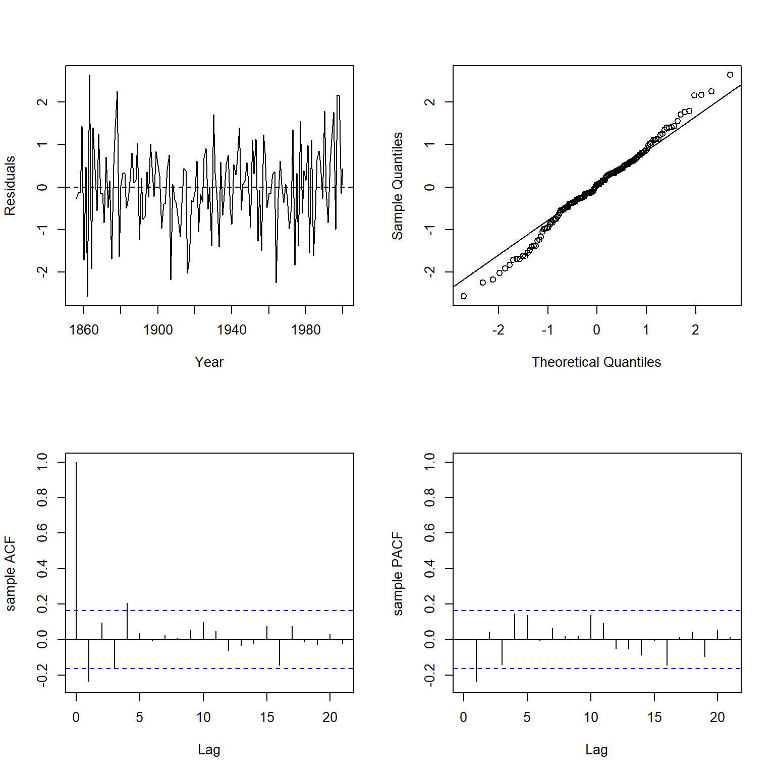
## 	Box-Ljung test
## 
## data:  y
## X-squared = 29.177, df = 21, p-value = 0.1098

There is no evidence of autocorrelation in the GLS model.

Let’s get the confidence interval on the estimated AR(1) autocorrelation coefficient (phi). Phi is the estimate of the correlation strength between consecutive measuresents, which in this case, indicates a clear serial dependence structure.

intervals(glmod1, which = 'var-cov')
## Approximate 95% confidence intervals
## 
##  Correlation structure:
##        lower      est.     upper
## Phi 0.509979 0.7109922 0.8383734
## 
##  Residual standard error:
##     lower      est.     upper 
## 0.1540717 0.2045720 0.2716249

Compare Models

Let’s compare the models using the model.sel() function from the MuMIn package. When comparing fits of models, all models should be fit to the same dataset. Because the wmod2 model introduced a lag term of the response variable temperature to the model, it was fit using a different set of predictors. However, let’s still compare the models.

library(MuMIn)
models <- model.sel(lmod, wmod1, wmod2, glmod1)
models <- data.frame(
  Model  = rownames(models),
  Class  = as.character(models$class),
  logLik = round(models$logLik, 1),
  AIC    = round(models$AIC, 1),
  delta  = round(models$delta, 1)
)
knitr::kable(models) %>%
kableExtra::kable_classic_2(full_width = F, position = 'center', html_font = 'Cambria')

Model	Class	logLik	AIC	delta
wmod2	lm	82.4	-140.8	0.0
glmod1	gls	65.1	-106.2	34.5
wmod1	lm	54.7	-87.7	53.0
lmod	lm	51.0	-80.3	60.4

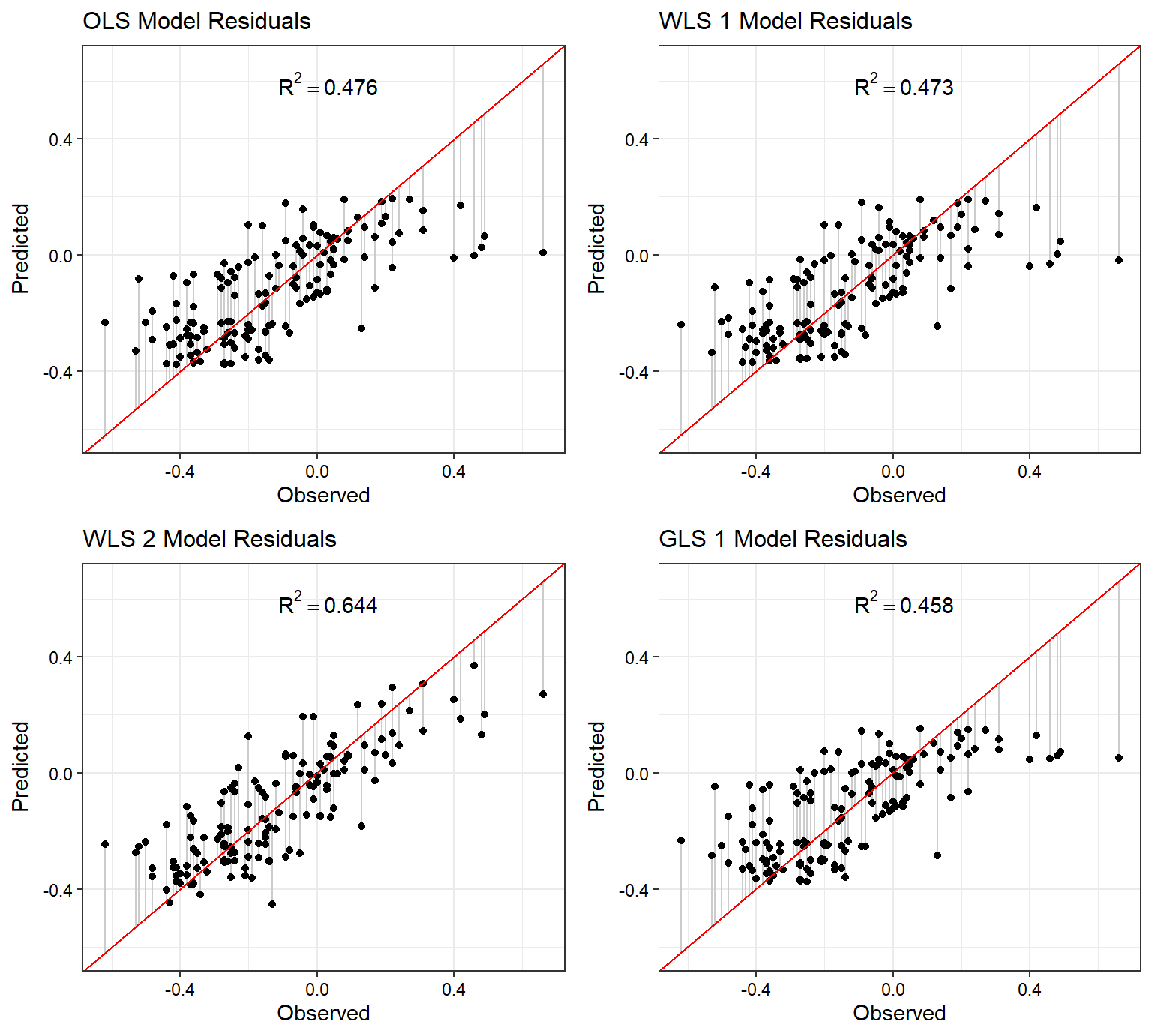
The wmod2 WLS model that utilized a lag term of the response variable as a predictor performs the best of the four models considered for this exercise. The glmod1 GLS model with an AR(1) error structure performs second best. The lmod OLS model is the lowest performing model.

Let’s plot the predicted versus observed values for each model, showing the model residuals for each observation.

p1 <- plot.linear.model(lmod, name = 'OLS')
p2 <- plot.linear.model(wmod1, name = 'WLS 1')
p3 <- plot.linear.model(wmod2, name = 'WLS 2')
p4 <- plot.linear.model(glmod1, name = 'GLS 1')

plots <- list(p1, p2, p3, p4)
cowplot::plot_grid(plotlist = plots)

Posted on:: April 17, 2024

Length:: 14 minute read, 2855 words

See Also: