Introduction

Heteroscedasticity refers to unequal scatter in the residuals or error term in regression analysis, where there is a systematic change in the spread of residuals over the range of measured values. This violates the assumption of constant variance in the errors, known as homoscedasticity, in ordinary least squares (OLS) regression. Heteroscedasticity can lead to less precise coefficient estimates and inflated p-values. When errors are independent, but not identically distributed, weighted least squares (WLS) regression can be used to address heteroscedasticity by placing more weight on observations with smaller error variance. Other methods to address heteroscedasticity include transforming the response variable or generalizing the model to allow for a less restrictive form of the error covariance matrix. Overall, it is important to detect and correct for heteroscedasticity to ensure the reliability of regression results.

In this blog post, we will explore methods to identify heteroscedasticity and work through an example to address non-constant variance using WLS regression. The analyses will be conducted using the R language for statistical computing and visualization.

Data

Let’s create a synthetic dataset containing heteroskedasticity.

# Generate data
set.seed(123)
n <- 500
x <- 5*rexp(n)
y <- 2*x + x*rnorm(n)

Let’s inspect a plot of the data.

summary(data.frame(x, y))

##        x                  y          
##  Min.   : 0.00413   Min.   : -4.506  
##  1st Qu.: 1.57575   1st Qu.:  2.223  
##  Median : 3.65402   Median :  6.389  
##  Mean   : 5.03551   Mean   : 10.368  
##  3rd Qu.: 7.13254   3rd Qu.: 14.005  
##  Max.   :36.05504   Max.   :112.141

plot(y ~ x, main = 'Plot of Y vs X')

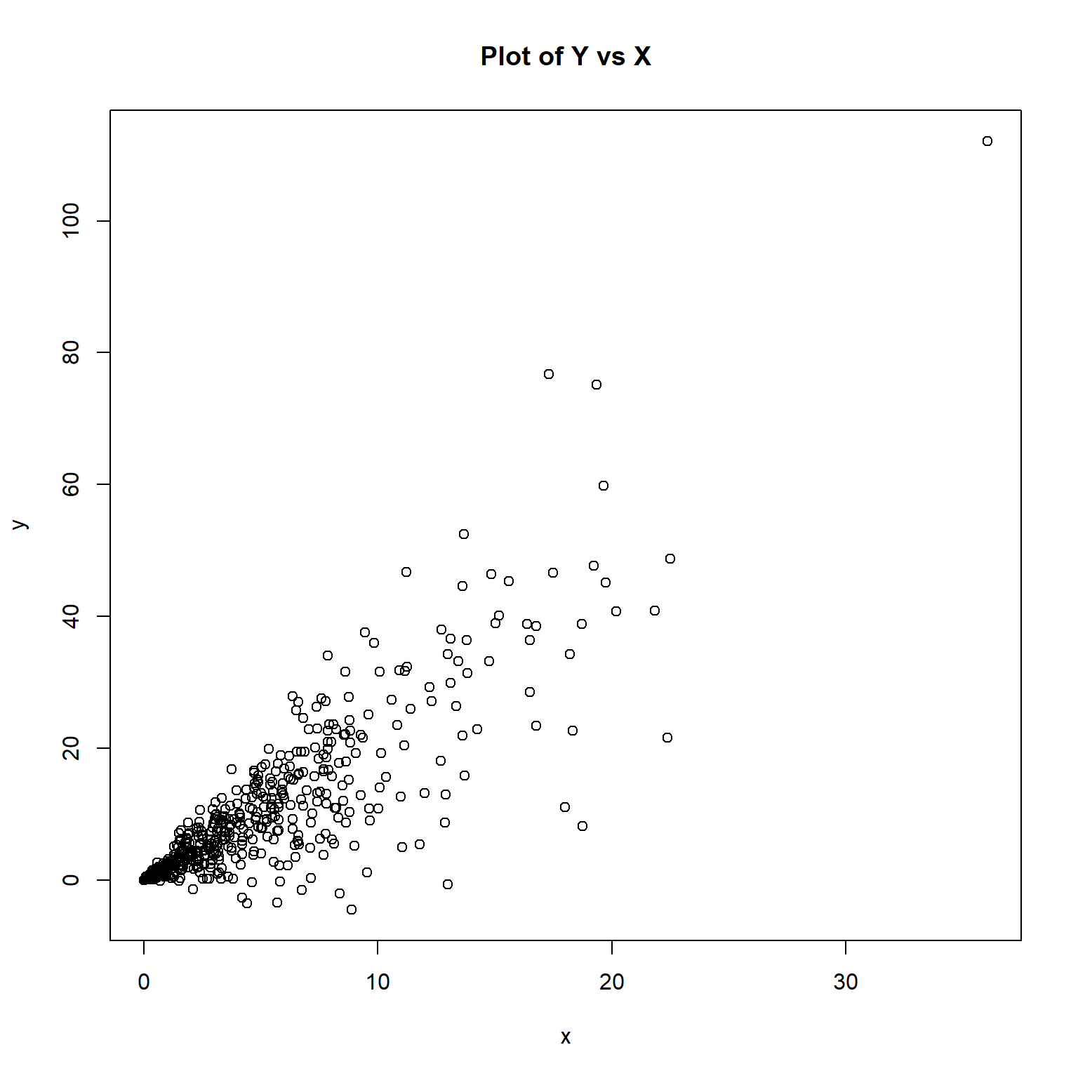
The plot of the data appear to exhibit heteroscedasticity, where the variance of the y-values increase with increasing values of x.

OLS Regression

Let’s perform OLS regression.

# Perform ordinary least squares regression
lmod <- lm(y ~ x)
summary(lmod)

## 
## Call:
## lm(formula = y ~ x)
## 
## Residuals:
##     Min      1Q  Median      3Q     Max 
## -32.444  -1.836   0.564   2.235  39.288 
## 
## Coefficients:
##             Estimate Std. Error t value Pr(>|t|)    
## (Intercept) -0.72901    0.44119  -1.652   0.0991 .  
## x            2.20371    0.06391  34.480   <2e-16 ***
## ---
## Signif. codes:  0 '***' 0.001 '**' 0.01 '*' 0.05 '.' 0.1 ' ' 1
## 
## Residual standard error: 6.748 on 498 degrees of freedom
## Multiple R-squared:  0.7048,	Adjusted R-squared:  0.7042 
## F-statistic:  1189 on 1 and 498 DF,  p-value: < 2.2e-16

A quick numerical test to check non-constant variance can be achieved by regressing the absolute value of the OLS residuals against the fitted values.

summary(lm(abs(lmod$residuals) ~ lmod$fitted.values))

## 
## Call:
## lm(formula = abs(lmod$residuals) ~ lmod$fitted.values)
## 
## Residuals:
##      Min       1Q   Median       3Q      Max 
## -16.5848  -1.7684  -0.2558   0.9077  26.3145 
## 
## Coefficients:
##                    Estimate Std. Error t value Pr(>|t|)    
## (Intercept)         0.64159    0.26194   2.449   0.0147 *  
## lmod$fitted.values  0.32941    0.01783  18.473   <2e-16 ***
## ---
## Signif. codes:  0 '***' 0.001 '**' 0.01 '*' 0.05 '.' 0.1 ' ' 1
## 
## Residual standard error: 4.149 on 498 degrees of freedom
## Multiple R-squared:  0.4066,	Adjusted R-squared:  0.4054 
## F-statistic: 341.2 on 1 and 498 DF,  p-value: < 2.2e-16

Based on the results of the regression, we conclude that heteroscedasticity is a problem in this model.

A difficulty with this approach is that it only tests for a linear trend in the variation. A formal test may be good at detecting a particular kind of non-constant variance, but have no power to detect another. One informal way of detecting heteroskedasticity is by creating a residual plot where you plot the least squares residuals against the independent variable or \(\hat{y}\) if it’s a multiple regression. These plots should display random residuals (no patterns) that are uncorrelated and uniform. If there is an evident pattern in the plot, then heteroskedasticity is present. Residual plots are more versatile because they are effective at revealing unanticipated structure.

# Inspect residuals
plot(lmod$residuals ~ x, main = 'OLS Residuals vs X')
abline(h = 0)

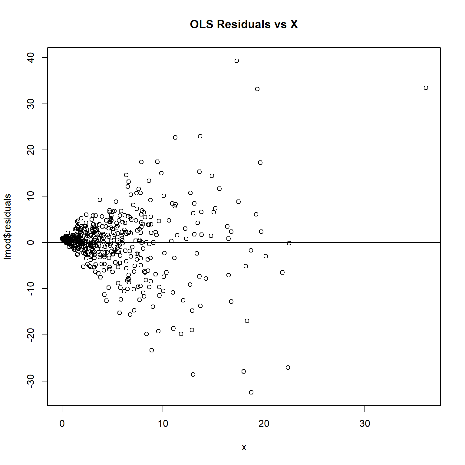
The plot exhibits a cone shaped pattern in the residuals. Note how the vertical range of the residuals increases as X increases.

A more formal, mathematical way of detecting heteroskedasticity is what is known as the Breusch-Pagan test. The Breusch-Pagan test is an likelihhod ratio test, based on the score of the log likelihood function, calculated under normality. It is a general test designed to detect any linear forms of heteroskedasticity. It tests the null hypothesis that heteroskedasticity is not present (i.e. homoskedastic) against the alternative hypothesis that heteroskedasticity is present. The test is implemented in the lmtest package.

# Breusch-Pagan test
lmtest::bptest(lmod)

## 
## 	studentized Breusch-Pagan test
## 
## data:  lmod
## BP = 145.74, df = 1, p-value < 2.2e-16

Because the p-value from the test is <0.001, we will reject the null hypothesis and conclude that heteroscedasticity is a problem in this model.

The Durbin Watson statistic is used as a test for checking autocorrelation in the residuals of a statistical regression analysis. The Durbin-Watson test evaluates errors for first-order autocorrelation where the null hypothesis is that the errors are uncorrelated and the alternative hypothesis is that first-order correlation exists. The test is implemented in the lmtest package.

# Durbin-Watson test
lmtest::dwtest(y ~ x)

## 
## 	Durbin-Watson test
## 
## data:  y ~ x
## DW = 1.9061, p-value = 0.1465
## alternative hypothesis: true autocorrelation is greater than 0

Because the p-value from the test is 0.147, we cannot reject the null hypothesis that the errors are uncorrelated.

WLS Regression

WLS can be used if the errors are uncorrelated, but the variance of the errors are not the same. WLS regression assigns weights to data points based on variance of fitted values to minimize the sum of weighted squared residuals. Correct weights can replace heteroscedasticity with homoscedasticity. Determining the source of heteroscedasticity may be challenging, so an alternative is estimating variances by using residuals as weights. High variability cases receive low weights, while low variability cases receive high weights.

WLS regression will be performed using the following steps:

• Regress the absolute values of the OLS residuals versus the OLS fitted values and store the fitted values from this regression. These fitted values are estimates of the error standard deviations.

• Calculate weights equal to \(1/fits^2\), where \(fits\) are the fitted values from the regression in the previous step.

• Refit the original regression model but using these weights in a WLS regression.

The first step is to calculate the weights.

# Define weights
wts <- 1/lm(abs(lmod$residuals) ~ lmod$fitted.values)$fitted.values^2

Now that the weights have been calculated, we can perform WLS regression.

# Perform weighted least squares regression
wmod <- lm(y ~ x, weights = wts)
summary(wmod)

## 
## Call:
## lm(formula = y ~ x, weights = wts)
## 
## Weighted Residuals:
##     Min      1Q  Median      3Q     Max 
## -3.4735 -0.7398  0.0470  0.7286  3.2086 
## 
## Coefficients:
##             Estimate Std. Error t value Pr(>|t|)    
## (Intercept) 0.003325   0.081290   0.041    0.967    
## x           2.026439   0.053150  38.127   <2e-16 ***
## ---
## Signif. codes:  0 '***' 0.001 '**' 0.01 '*' 0.05 '.' 0.1 ' ' 1
## 
## Residual standard error: 1.148 on 498 degrees of freedom
## Multiple R-squared:  0.7448,	Adjusted R-squared:  0.7443 
## F-statistic:  1454 on 1 and 498 DF,  p-value: < 2.2e-16

The residual standard error can be calculated manually using the following:

# Manually calculate residual standard error
k <- length(wmod$coefficients) - 1   # subtract one to ignore intercept
n <- length(wmod$residuals)
SSE <- sum(wts * (wmod$residuals)**2)
sqrt(SSE/(n - (1 + k)))     # residual Standard Error

## [1] 1.147858

The WLS model has a residual standard error of 1.148 compared to 6.748 in the OLS regression model. This indicates that the predicted values produced by the WLS model are much closer to the actual observations compared to the predicted values produced by the OLS regression model.

As an alternative approach, WLS regression can be performed manually as shown below.

# Manually perform weighted least squares regression
v <- sqrt(wts)
x2 <- x*v
y2 <- y*v
wmod2 <- lm(y2 ~ 0 + v + x2)
summary(wmod2)

## 
## Call:
## lm(formula = y2 ~ 0 + v + x2)
## 
## Residuals:
##     Min      1Q  Median      3Q     Max 
## -3.4735 -0.7398  0.0470  0.7286  3.2086 
## 
## Coefficients:
##    Estimate Std. Error t value Pr(>|t|)    
## v  0.003325   0.081290   0.041    0.967    
## x2 2.026439   0.053150  38.127   <2e-16 ***
## ---
## Signif. codes:  0 '***' 0.001 '**' 0.01 '*' 0.05 '.' 0.1 ' ' 1
## 
## Residual standard error: 1.148 on 498 degrees of freedom
## Multiple R-squared:  0.7984,	Adjusted R-squared:  0.7976 
## F-statistic: 986.1 on 2 and 498 DF,  p-value: < 2.2e-16

We can use the following function to calculate the r-squared value for each regression analysis.

# Function to get r-squared
get_r2 <- function(x, weight = FALSE) {
  observed <- x$resid + x$fitted
  if (weight) {
    SSe <- sum(x$w*(x$resid)^2)
    SSt <- sum(x$w*(observed - weighted.mean(observed,x$w))^2)
  }
  else {
    SSe <- sum((x$resid)^2)
    SSt <- sum((observed - mean(observed))^2)
  }
  value <- 1 - SSe/SSt
  return(value)  
}

# Get r-squared values
get_r2(lmod)

## [1] 0.7047812

get_r2(wmod, weight = TRUE)

## [1] 0.7448317

The WLS model has a r-squared of 0.7448 compared to 0.7048 for the OLS regression model. This indicates that the WLS model is able to explain more of the variance in Y compared to the OLS regression model.

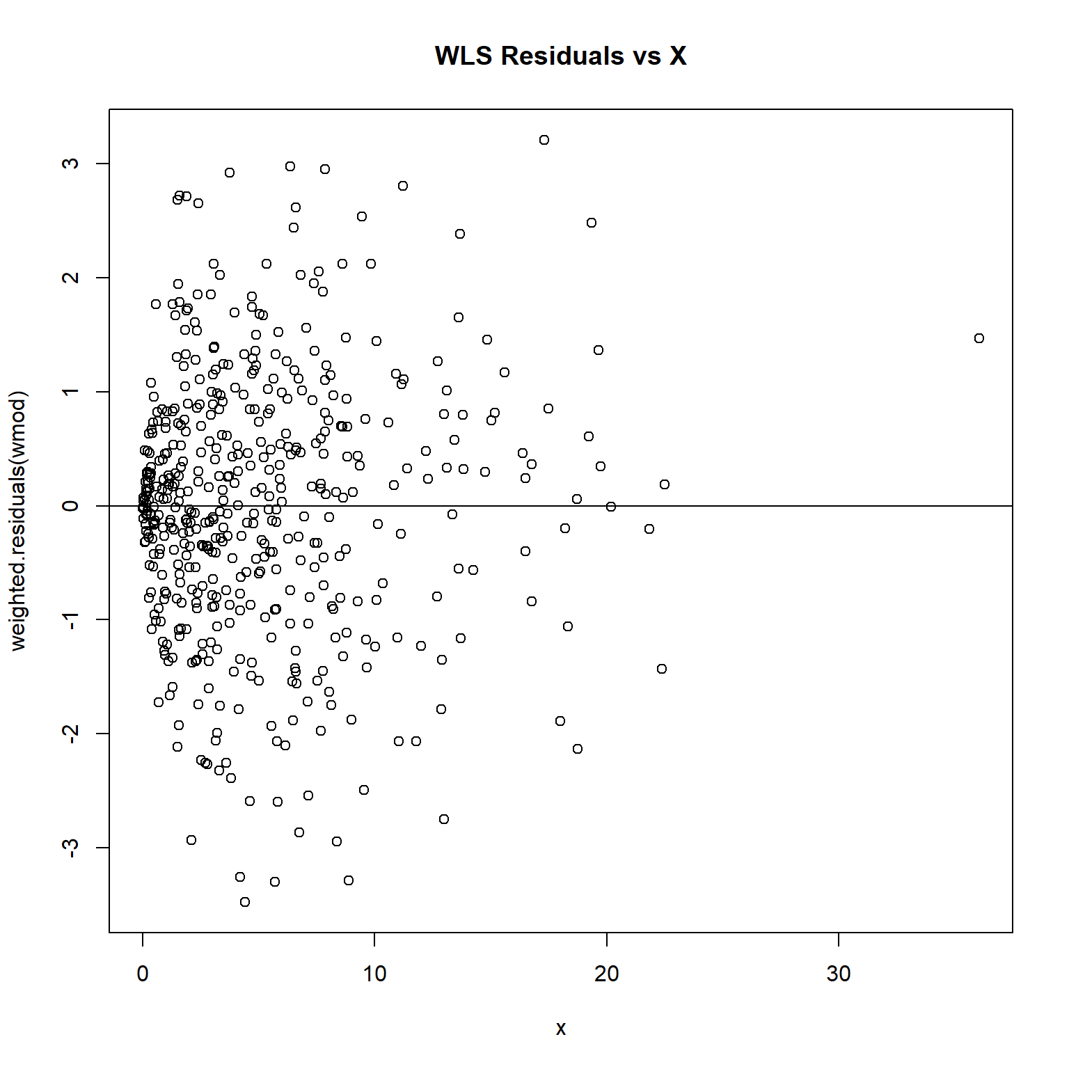
The weighted residuals can be obtained by using the weighted.residuals() function or by multiplying the model residuals by the square-root of the weights, \(\sqrt{(w_i)}\varepsilon_i\). Let’s plot the weighted residuals against X.

# Inspect residuals
plot(weighted.residuals(wmod) ~ x, main = 'WLS Residuals vs X')
abline(h = 0)

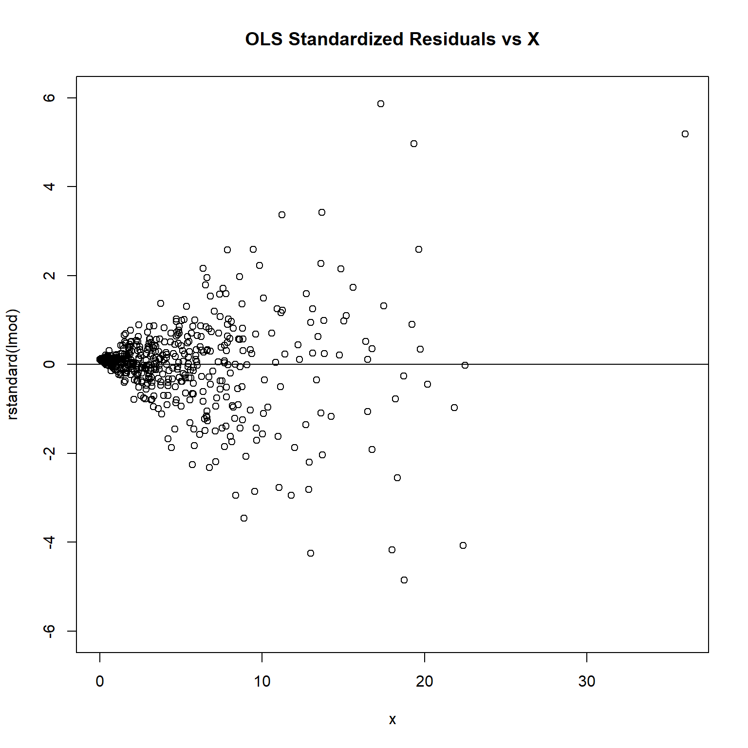
To see if the weights are chosen properly to fix the heteroscedastic problem, we can plot the standardized or studentized residuals and see if the points scatter evenly around the zero line.

plot(rstandard(lmod) ~ x, ylim = c(-6, 6), main = 'OLS Standardized Residuals vs X')
abline(h = 0)

plot(rstandard(wmod) ~ x, ylim = c(-6, 6), main = 'WLS Standardized Residuals vs X')
abline(h = 0)

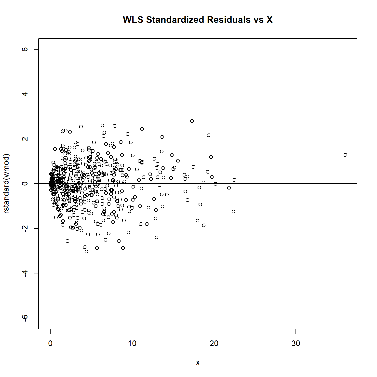
The plot of standardized residuals against the predictor shows the same pattern as the residual plot implying that heterogeneity is likely to be due a relationship between variance and X. That is, an increase in X is associated with an increase in variance.

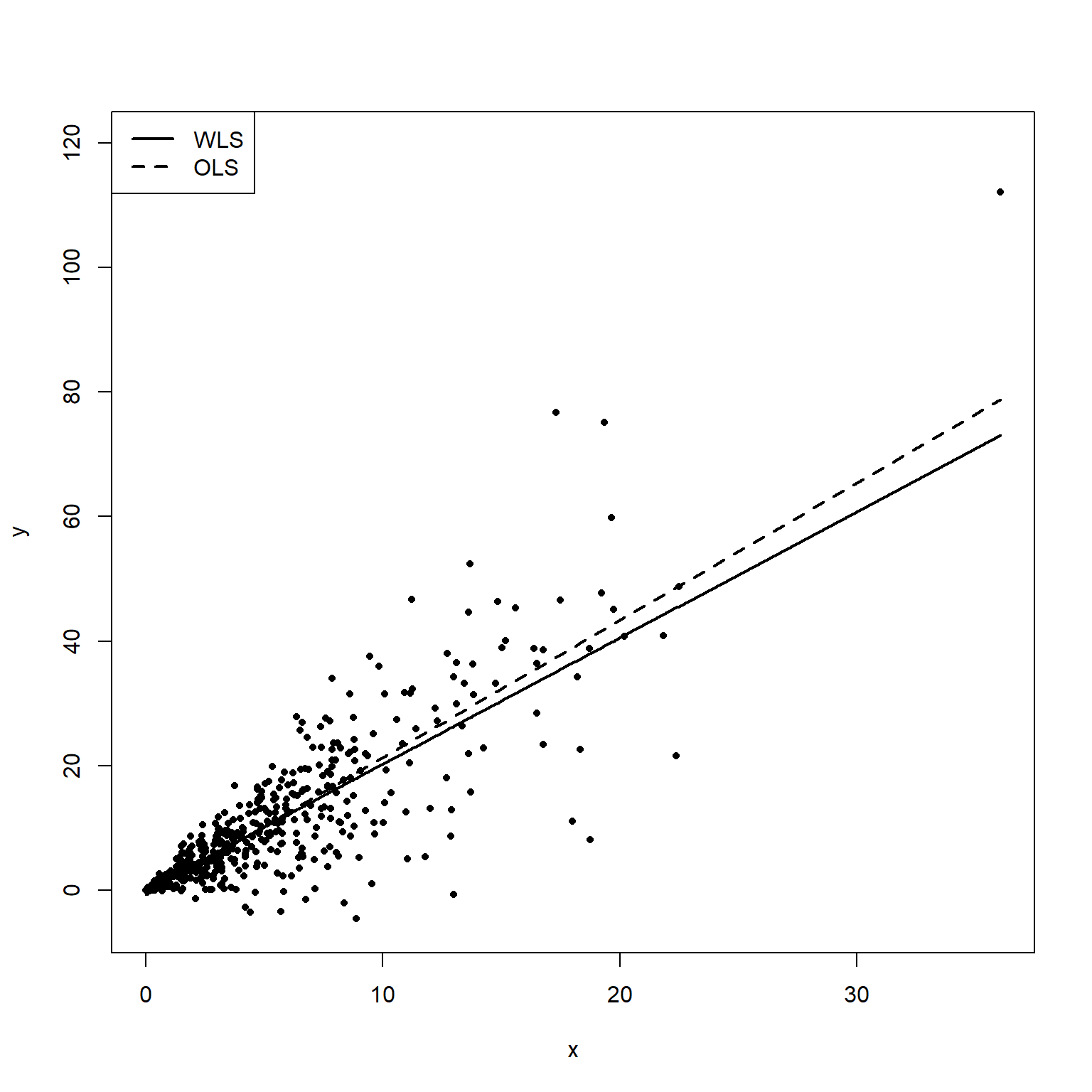
The following plot shows both the OLS fitted line (dashed) and WLS fitted line (solid). The WLS fit is more heavily weighted on the middle points where the variance is lower.

# Get predicted values
lmod.pred <- lmod$fitted.values
wmod.pred <- wmod$fitted.values

# Plot data and fits
plot(x, y, pch = 16, cex = 0.7, ylim = c(-5, 120))
points(sort(x), sort(lmod.pred), type = 'l', lty = 2, lwd = 2)
points(sort(x), sort(wmod.pred), type = 'l', lty = 1, lwd = 2)
legend('topleft', c('WLS', 'OLS'), lty = c(1, 2), lwd = 2)

Let’s plot the data and regression analyses where the variance is small (X data <1).

idx <- x<1
plot(x[idx], y[idx], pch = 16, cex = 0.8, ylim = c(-1, 3))
points(sort(x[idx]), sort(lmod.pred[idx]), type = 'l', lty = 2, lwd = 2)
points(sort(x[idx]), sort(wmod.pred[idx]), type = 'l', lty = 1, lwd = 2)
legend('topleft', c('WLS', 'OLS'), lty = c(1, 2), lwd = 2)

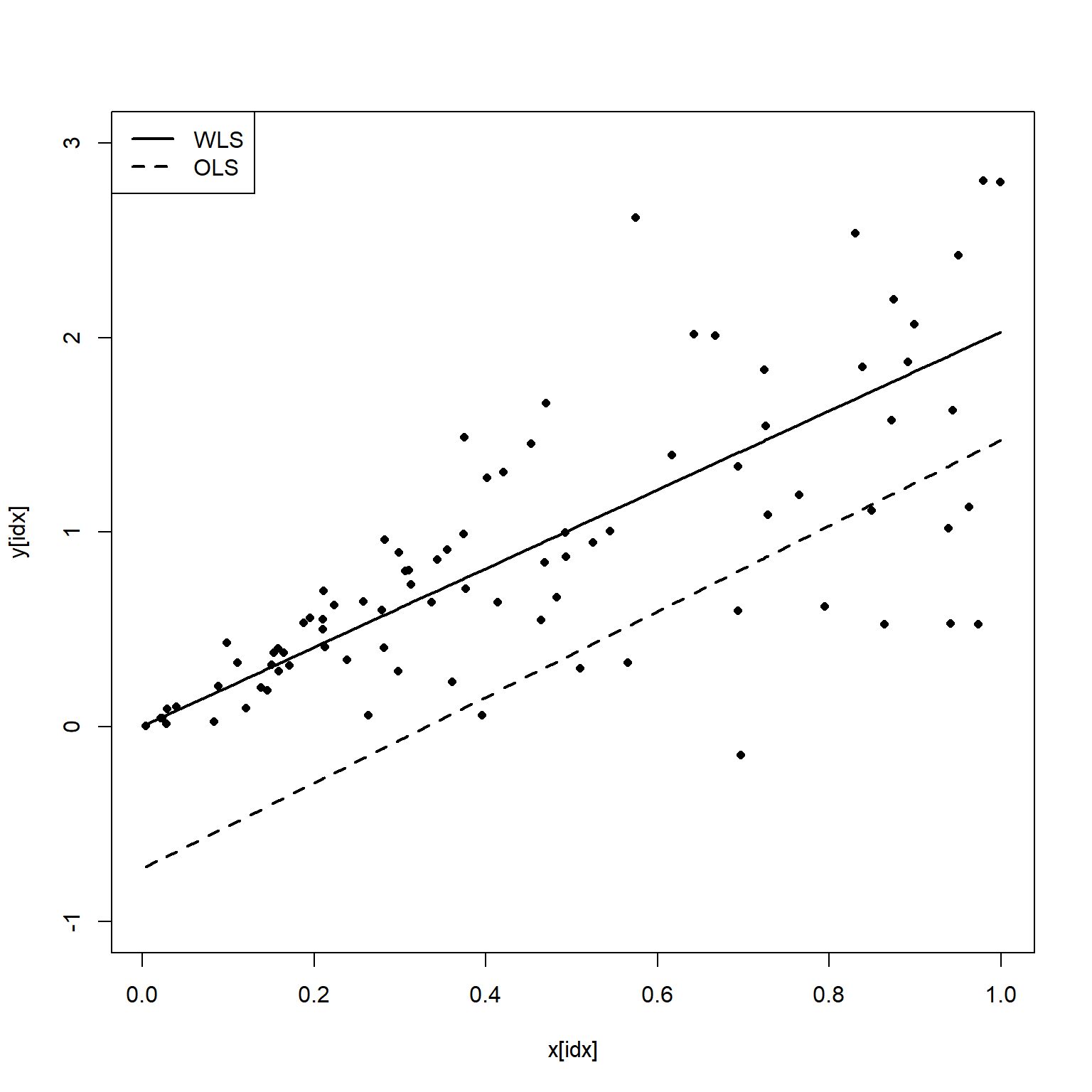
Based on this plot, we see that the OLS estimate misses the data badly where the variance of Y is small.

Conclusions

Heteroscedasticity in regression analysis refers to varying levels of scatter in the residuals, indicating a systematic change in the spread of errors across different values. It can be detected through plots or formal statistical tests. Its presence affects OLS estimators and standard errors, leading to biased estimates and misleading results. To address for heteroscedasticity, WLS can be used to obtain parameter estimates, involving transforming the model to be homoskedastic by estimating a variance function and using the square root of the estimates as weights. This results in smaller standard errors and more precise estimators. WLS can be used if the errors are uncorrelated, but the variance of the errors are not the same.

Identifying and addressing heteroscedasticity requires understanding its various causes and may involve complex subject-area knowledge. Severe cases often necessitate remedial actions. However, if the main objective is predicting the total dependent variable amount rather than estimating particular independent variable effects, correcting for non-constant variance may be unnecessary. If the sample size is large enough, the variance of the OLS estimator may still be sufficiently small to obtain precise estimates.