Nonparametric Two-Way ANOVA
By Charles Holbert
April 16, 2022
Introduction
Often data from more than two groups within a single factor needs to be evaluated, usually on the basis of a representative value from each group. For uncensored data, comparisons among groups are made using the parametric analysis of variance (ANOVA) and the nonparametric Kruskal-Wallis (KW) test. These tests determine whether the groups essentially belong to the same underlying population, or whether there are significant differences between the group distributions. This is the simplest type of ANOVA design and is called one-way ANOVA. Two-way ANOVA is when two factors or variables potentially affect the response variable. For conventional two-way ANOVA with several observations or data values for each combination of factors, it is possible to test for factor interaction. Factor interaction refers to the case where each factor not only exerts an effect on the response variable (described as main effects), but also may interact with the other factor or factors to exert additional joint effects on the response variable (known as interaction effects)
If the data meet normality and homoscedasticity (i.e., equality of variance) requirements of parametric ANOVA, methods are available for computing two-way ANOVA. However, the KW test for nonparametric ANOVA cannot be directly extended to the case where there are two or more factors as is done with parametric two-way ANOVA. Instead, a nonparametric approximate approach is to transform the data values. One method that is not unduly affected by violations of the normality and homoscedasticity assumptions of parametric ANOVA is to transform the data values to their ranks, and then compute a parametric two-way ANOVA on the data ranks. This rank transformation procedure can be used to determine whether the ranks differ from group to group. Post-hoc comparisons can be performed on the data ranks to determine which groups are different from each other. An alternative approach is to use ordinal logistic regression to provide general contrasts on the log odds ratio scale (Harrell 2015).
In this post, we will evaluate whether sample depth and/or site location affect arsenic concentrations measured in soil. To address non-normality and heteroscedasticity, two-way ANOVA will be performed using the rank-transformation of the data values.
Data
Arsenic concentrations were measured in soil from two depth intervals, shallow (SS) and deep (SB), at five sites (RA1 through RA5). We would like to determine whether arsenic concentrations in soil not only exhibit spatial variability between site locations but also may be affected by sample depth. This constitutes a two-way ANOVA problem, with one factor as location (represented by the five sites) and the second factor as matrix (represented by the two soil sample depths).
First, let’s load the data from the comma-delimited file and then make the LOCATION and MATRIX variables ordered factors.
# Load libraries
library(dplyr)
library(car)


# Load data
dat <- read.csv('data/Soil_Arsenic.csv', header = T)
dat$LOGDATE <- as.POSIXct(dat$LOGDATE, format = '%m/%d/%Y')

# Make matrix variable ordered factor
dat$MATRIX <- factor(
  dat$MATRIX, ordered = TRUE,
  levels = c('SS', 'SB')
)

# Make matrix variable ordered factor
dat$LOCATION <- factor(
  dat$LOCATION, ordered = TRUE,
  levels = c('RA1', 'RA2', 'RA3', 'RA4', 'RA5')
)

str(dat)
## 'data.frame':	266 obs. of  11 variables:
##  $ LOCATION: Ord.factor w/ 5 levels "RA1"<"RA2"<"RA3"<..: 3 3 3 3 3 3 3 3 3 3 ...
##  $ SACODE  : chr  "N" "N" "N" "N" ...
##  $ LOGDATE : POSIXct, format: "2019-08-15" "2019-08-15" ...
##  $ MATRIX  : Ord.factor w/ 2 levels "SS"<"SB": 1 1 1 1 1 1 1 1 1 1 ...
##  $ MEDIA   : chr  "Soil" "Soil" "Soil" "Soil" ...
##  $ DILUTION: int  1 1 1 1 1 1 1 1 1 1 ...
##  $ PARAM   : chr  "Arsenic" "Arsenic" "Arsenic" "Arsenic" ...
##  $ DETECTED: chr  "Y" "Y" "Y" "Y" ...
##  $ RESULT  : num  2.95 2.83 2.96 2.55 4.02 3.7 3.52 3.03 3.27 3.52 ...
##  $ MDL     : num  1 0.8 0.8 0.8 0.8 1 0.8 0.8 0.8 0.8 ...
##  $ UNITS   : chr  "ppb" "ppb" "ppb" "ppb" ...
We see that the data contain 266 observations and 11 variables. Let’s create a frequency table to see how the observations are distributed between the MATRIX and LOCATION groups.
# Create frequency table
with(dat, table(LOCATION, MATRIX))
##         MATRIX
## LOCATION SS SB
##      RA1 25 23
##      RA2 25 11
##      RA3 25 25
##      RA4 25  7
##      RA5 25 75
For the SS soil depth, there are 25 samples per location. For the SB soil depth, the sample size ranges from 7 for RA4 to 75 for RA5. Thus, we have an unbalanced design. When sample sizes are substantially dissimilar, accurate interpretation of the main and interaction effects of the factors on the response variable becomes complicated, and the unequal sample sizes have a confounding effect on the factors.
Let’s calculate summary statistics for each data group.
# Compute summary statistics
dat %>%
  group_by(MATRIX, LOCATION) %>%
  summarise(
    count = n(),
    mean = round(mean(RESULT, na.rm = TRUE), 2),
    median = round(median(RESULT, na.rm = TRUE), 2),
    sd = round(sd(RESULT, na.rm = TRUE), 2),
    cv = round(sd/mean, 2),
  ) %>%
  ungroup()
## # A tibble: 10 x 7
##    MATRIX LOCATION count  mean median    sd    cv
##    <ord>  <ord>    <int> <dbl>  <dbl> <dbl> <dbl>
##  1 SS     RA1         25  6.37   6.12  1.57  0.25
##  2 SS     RA2         25  8.54   8.48  1.46  0.17
##  3 SS     RA3         25  3.59   3.27  1.01  0.28
##  4 SS     RA4         25  7.21   7.17  2.04  0.28
##  5 SS     RA5         25  6.6    6.68  0.8   0.12
##  6 SB     RA1         23  4.82   3.62  3.01  0.62
##  7 SB     RA2         11  4.58   4.57  2.83  0.62
##  8 SB     RA3         25  3.1    3.09  0.61  0.2
##  9 SB     RA4          7  4.57   4.2   3.04  0.67
## 10 SB     RA5         75  6.33   6.24  0.64  0.1
As expected, the central tendency and spread in arsenic concentrations vary between sample depth and location. The highest variability in concentration is associated with samples collected from the SB soil depth at locations RA1, RA2, and RA4.
Let’s visually inspect the data using box plots and an interaction plot. Box plots show the central tendency, degree of symmetry, range of variation, and potential outliers of a data set. The upper value of the box represents the 75th percentile for the data and the lower value of the box is the 25th percentile for the data. Thus, 50 percent of the data fall within the box. The top of the whisker represents the 75th percentile plus 1.5 times the interquartile range (IQR), where the IQR is the 75th percentile minus the 25th percentile. The bottom of the whisker is the 25th percentile minus 1.5 times the IQR. Any value outside of this range is considered a potential statistical outlier, which is represented by a dot on the plot. An interaction plot displays the levels of one variable on the x-axis and has a separate line for the means of each level of the other variable. The y-axis is the dependent or response variable. We will use the R package ggpubr to create the plots.
# Load library
library(ggpubr)
library(cowplot)

# Box plot
p1 <- ggboxplot(
  dat, x = 'LOCATION', y = 'RESULT', fill = 'MATRIX',
  palette = c('#257ABA', '#C9B826')
)

# Line plot
p2 <- ggline(
  dat, x = 'LOCATION', y = 'RESULT', color = 'MATRIX',
  add = c('mean_se', 'dotplot'), size = 1,
  palette = c('#257ABA', '#C9B826'))

plot_grid(p1, p2, ncol = 1, align = 'v')
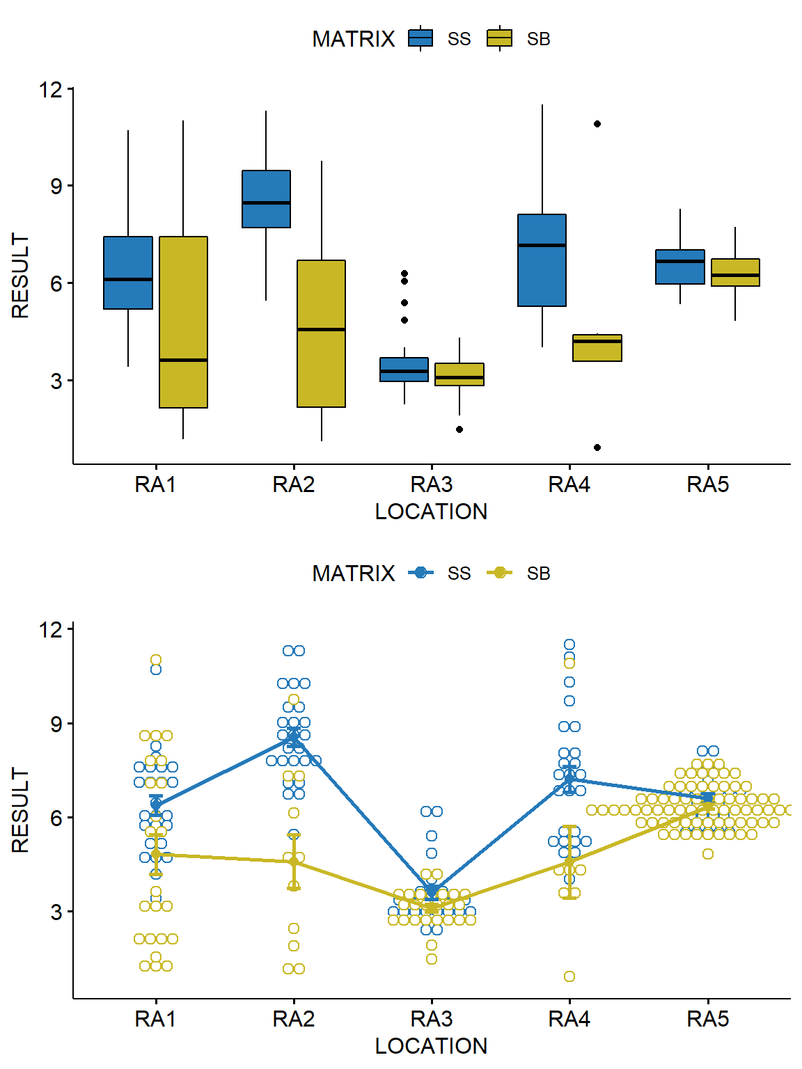
Based on these plots, it appears that arsenic concentrations are significantly different across the two soil depths for locations RA2 and RA4.
Two-Way ANOVA
Two-way ANOVA with replication can be used to test three null hypotheses: that the means of observations grouped by one factor are the same; that the means of observations grouped by the other factor are the same; and that there is no interaction between the two factors. When the interaction term is significant, each factor is evaluated separately using a one-way ANOVA.
Unbalanced two-way ANOVA is generally performed using Type-III sum of squares (SS). Estimates based on Type-III SS tell us how much of the residual variability in the response variable Y can be accounted for by factor A after having taken into account factor B and the A:B interaction, and how much of the residual variability in Y can be accounted for by factor B after having taken into account factor A and the A:B interaction. When using Type-III SS, factors should be set to use effects coding rather than relying on the default treatment codes. This can be done by adding the appropriate sum to zero contrasts as an argument to R’s aov function.
Let’s first perform two-way ANOVA on the original data.
# ANOVA procedure on original data
aov.org <- aov(
  RESULT ~ MATRIX * LOCATION, data = dat,
  contrasts = list(
    MATRIX = 'contr.sum',
    LOCATION = 'contr.sum'
  )
)
Anova(aov.org, type = 'III')
## Anova Table (Type III tests)
##
## Response: RESULT
##                 Sum Sq  Df   F value    Pr(>F)
## (Intercept)     5851.4   1 2399.7704 < 2.2e-16 ***
## MATRIX           149.7   1   61.4003 1.248e-13 ***
## LOCATION         339.5   4   34.8078 < 2.2e-16 ***
## MATRIX:LOCATION   93.0   4    9.5304 3.377e-07 ***
## Residuals        624.2 256
## ---
## Signif. codes:  0 '***' 0.001 '**' 0.01 '*' 0.05 '.' 0.1 ' ' 1
Now, let’s perform two-way ANOVA on the log-transformed data.
# ANOVA procedure on log-transformed data
aov.log <- aov(
  log(RESULT) ~ MATRIX * LOCATION, data = dat,
  contrasts = list(
    MATRIX = 'contr.sum',
    LOCATION = 'contr.sum'
  )
)
Anova(aov.log, type = 'III')
## Anova Table (Type III tests)
##
## Response: log(RESULT)
##                 Sum Sq  Df  F value    Pr(>F)
## (Intercept)     479.08   1 4379.867 < 2.2e-16 ***
## MATRIX            8.24   1   75.355 4.684e-16 ***
## LOCATION         14.40   4   32.914 < 2.2e-16 ***
## MATRIX:LOCATION   4.63   4   10.571 6.079e-08 ***
## Residuals        28.00 256
## ---
## Signif. codes:  0 '***' 0.001 '**' 0.01 '*' 0.05 '.' 0.1 ' ' 1
Finaly, let’s perform two-way ANOVA on the rank-transformed data. Ranking is one of many procedures used to transform data that do not meet the assumptions of normality. Conover and Iman (1981) provided a review of the four main types of rank transformations. One method replaces each original data value by its rank (from 1 for the smallest to N for the largest, where N is the combined data sample size). This rank-based procedure has been recommended as being robust to non-normal errors, resistant to outliers, and highly efficient for many distributions.
# ANOVA procedure on rank-transformed data
aov.rnk <- aov(
  rank(RESULT) ~ MATRIX * LOCATION, data = dat,
  contrasts = list(
    MATRIX = 'contr.sum',
   LOCATION = 'contr.sum'
  )
)
Anova(aov.rnk, type = 'III')
## Anova Table (Type III tests)
##
## Response: rank(RESULT)
##                  Sum Sq  Df F value    Pr(>F)
## (Intercept)     2911804   1 936.506 < 2.2e-16 ***
## MATRIX           168683   1  54.252 2.419e-12 ***
## LOCATION         442327   4  35.566 < 2.2e-16 ***
## MATRIX:LOCATION  101199   4   8.137 3.431e-06 ***
## Residuals        795960 256
## ---
## Signif. codes:  0 '***' 0.001 '**' 0.01 '*' 0.05 '.' 0.1 ' ' 1
The results indicate that soil depth (MATRIX), site location (LOCATION), and the interaction between depth and location (MATRIX:LOCATION) are statistically significant (p-value < 0.05). Let’s inspect the grand means and the group means.
model.tables(aov.org, type = "means", se = TRUE)
## Tables of means
## Grand mean
##
## 5.840902
##
##  MATRIX
##          SS      SB
##       6.463   5.289
## rep 125.000 141.000
##
##  LOCATION
##        RA1    RA2    RA3    RA4     RA5
##      5.567  7.069  3.312  6.265   6.659
## rep 48.000 36.000 50.000 32.000 100.000
##
##  MATRIX:LOCATION
##       LOCATION
## MATRIX RA1   RA2   RA3   RA4   RA5
##    SS   6.37  8.54  3.59  7.21  6.60
##    rep 25.00 25.00 25.00 25.00 25.00
##    SB   4.82  4.58  3.10  4.57  6.33
##    rep 23.00 11.00 25.00  7.00 75.00
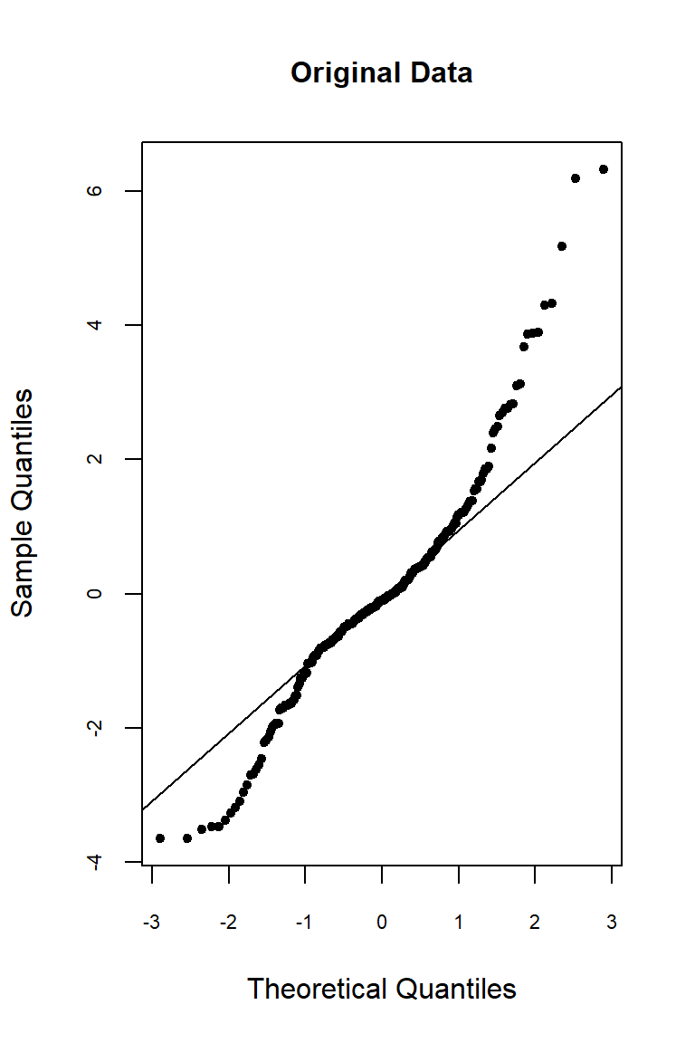
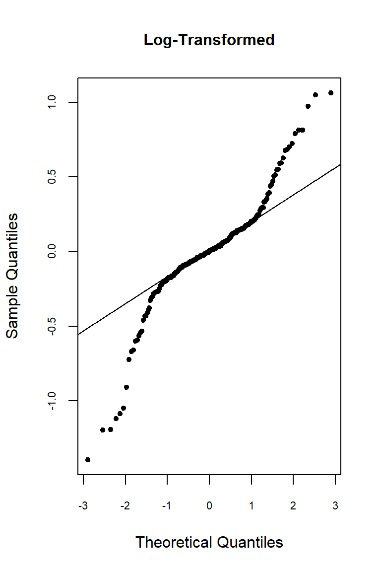
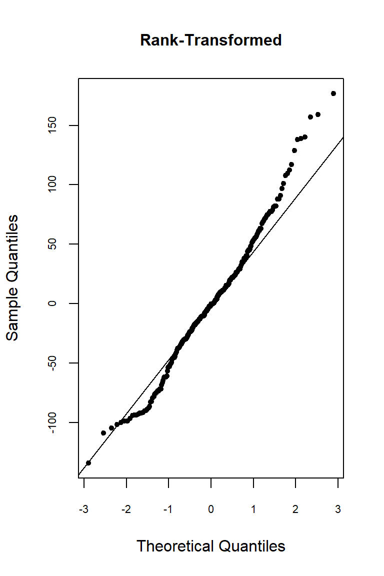
Let’s inspect the residuals from each model for normality. The residuals from the models using the orginal data and the log-transformed data deviate signficantly form nonmality. Residuals from the rank-transformed data model appear much better, although ranks aren’t expected to be normally distributed; barring any ties, ranks within any given group act like a sample without replacement from a discrete uniform distribution.
res.org = aov.org$resid
res.log = aov.log$resid
res.rnk = aov.rnk$resid
qqnorm(
  res.org, pch = 20, main = "Original Data",
  cex.lab = 1, cex.axis = 0.7, cex.main = 1
)
qqline(res.org)

qqnorm(
  res.log, pch = 20, main = "Log-Transformed",
  cex.lab = 1, cex.axis = 0.7, cex.main = 1
)
qqline(res.log)

qqnorm(
  res.rnk, pch = 20, main = "Rank-Transformed",
  cex.lab = 1, cex.axis = 0.7, cex.main = 1
)
qqline(res.rnk)
Now, let’s inspect the residuals versus the fitted values as a visual check for homogeneity of variances.
plot(aov.org, 1, main = "Original Data")
plot(aov.log, 1, main = "Log-Transformed")
plot(aov.rnk, 1, main = "Rank-Transformed")
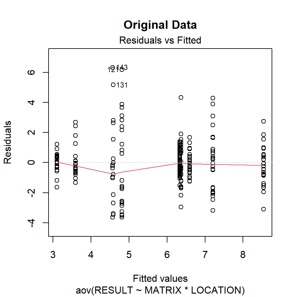
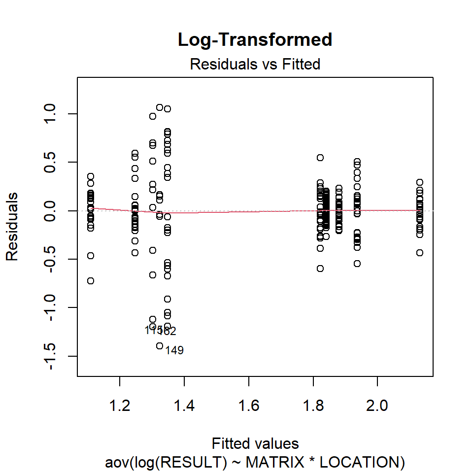
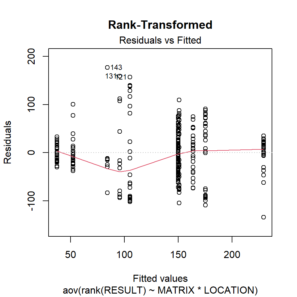
There is no evident relationships between residuals and the fitted values. Several points are identified as outliers, which can affect normality and homogeneity of variance.
Nature of Interactions
Let’s inspect the nature of the interactions using the R package emmeans. The emmeans package includes functions to facilitate post-hoc comparisons and contrast analysis. Let’s compare LOCATION separately for each MATRIX. The first thing to investigate is the significance of the interaction. If it is nonsignificant, we can focus on the main effects. However, if the interaction is significant, the main effects will not be helpful, as we will need to explore when each factor is significant given the levels of the other factor.
# Compute estimated marginal means for factor combinations
library(emmeans)
emmeans(aov.rnk, pairwise ~ LOCATION | MATRIX)
## $emmeans
## MATRIX = SS:
##  LOCATION emmean    SE  df lower.CL upper.CL
##  RA1       150.7 11.15 256    128.8    172.7
##  RA2       229.3 11.15 256    207.4    251.3
##  RA3        52.2 11.15 256     30.2     74.1
##  RA4       175.1 11.15 256    153.2    197.1
##  RA5       163.7 11.15 256    141.7    185.7
##
## MATRIX = SB:
##  LOCATION emmean    SE  df lower.CL upper.CL
##  RA1       105.0 11.63 256     82.1    127.9
##  RA2        95.7 16.81 256     62.6    128.8
##  RA3        37.2 11.15 256     15.2     59.1
##  RA4        84.0 21.08 256     42.5    125.5
##  RA5       150.0  6.44 256    137.3    162.7
##
## Results are given on the rank (not the response) scale.
## Confidence level used: 0.95
##
## $contrasts
## MATRIX = SS:
##  contrast  estimate   SE  df t.ratio p.value
##  RA1 - RA2   -78.62 15.8 256  -4.985  <.0001
##  RA1 - RA3    98.54 15.8 256   6.248  <.0001
##  RA1 - RA4   -24.40 15.8 256  -1.547  0.5328
##  RA1 - RA5   -12.98 15.8 256  -0.823  0.9234
##  RA2 - RA3   177.16 15.8 256  11.233  <.0001
##  RA2 - RA4    54.22 15.8 256   3.438  0.0061
##  RA2 - RA5    65.64 15.8 256   4.162  0.0004
##  RA3 - RA4  -122.94 15.8 256  -7.795  <.0001
##  RA3 - RA5  -111.52 15.8 256  -7.071  <.0001
##  RA4 - RA5    11.42 15.8 256   0.724  0.9508
##
## MATRIX = SB:
##  contrast  estimate   SE  df t.ratio p.value
##  RA1 - RA2     9.29 20.4 256   0.455  0.9911
##  RA1 - RA3    67.86 16.1 256   4.212  0.0003
##  RA1 - RA4    21.02 24.1 256   0.873  0.9065
##  RA1 - RA5   -44.96 13.3 256  -3.383  0.0073
##  RA2 - RA3    58.57 20.2 256   2.903  0.0325
##  RA2 - RA4    11.73 27.0 256   0.435  0.9925
##  RA2 - RA5   -54.26 18.0 256  -3.014  0.0235
##  RA3 - RA4   -46.84 23.8 256  -1.964  0.2865
##  RA3 - RA5  -112.83 12.9 256  -8.762  <.0001
##  RA4 - RA5   -65.99 22.0 256  -2.994  0.0249
##
## Note: contrasts are still on the rank scale
## P value adjustment: tukey method for comparing a family of 5 estimates
We see that the effect of MATRIX depends on the levels of LOCATION and vice versa. The next step is to determine the nature of the interaction. Let’s perform something akin to a one-way ANOVA for MATRIX within each level of LOCATION. However, the F-test will utilize all of the information from the full two-way factorial model.
em_out_category <- emmeans(aov.rnk,  ~ MATRIX | LOCATION)
print(em_out_category)
## LOCATION = RA1:
##  MATRIX emmean    SE  df lower.CL upper.CL
##  SS      150.7 11.15 256    128.8    172.7
##  SB      105.0 11.63 256     82.1    127.9
##
## LOCATION = RA2:
##  MATRIX emmean    SE  df lower.CL upper.CL
##  SS      229.3 11.15 256    207.4    251.3
##  SB       95.7 16.81 256     62.6    128.8
##
## LOCATION = RA3:
##  MATRIX emmean    SE  df lower.CL upper.CL
##  SS       52.2 11.15 256     30.2     74.1
##  SB       37.2 11.15 256     15.2     59.1
##
## LOCATION = RA4:
##  MATRIX emmean    SE  df lower.CL upper.CL
##  SS      175.1 11.15 256    153.2    197.1
##  SB       84.0 21.08 256     42.5    125.5
##
## LOCATION = RA5:
##  MATRIX emmean    SE  df lower.CL upper.CL
##  SS      163.7 11.15 256    141.7    185.7
##  SB      150.0  6.44 256    137.3    162.7
##
## Results are given on the rank (not the response) scale.
## Confidence level used: 0.95
Next, we pipe this object into the pairs() function and use the joint = TRUE option in the test() function to get the joint test of significance (i.e., the ANOVA F-test). The test function is similar to running multiple one-way ANOVAs, except we are using the error term from the full two-way factorial model. The results include the following:
- df1: degrees of freedom between groups
- df2: degrees of freedom within groups
- F.ratio: F statistic for MATRIX within each level of LOCATION
- p.value: probability of a Type-I error for each category
em_out_category %>%
  pairs() %>%
  test(joint = TRUE)
##  LOCATION df1 df2 F.ratio p.value
##  RA1        1 256   8.046  0.0049
##  RA2        1 256  43.861  <.0001
##  RA3        1 256   0.907  0.3418
##  RA4        1 256  14.604  0.0002
##  RA5        1 256   1.134  0.2879
We find that MATRIX is significant for RA1, RA2, and RA4; the effect of MATRIX is not significant for RA3 and RA5. Because MATRIX only has two levels, we do not need to do any further pairwise comparisons. The following code tells us which pairwise difference led to the significant joint F-test.
pairs(em_out_category)
## LOCATION = RA1:
##  contrast estimate   SE  df t.ratio p.value
##  SS - SB      45.7 16.1 256   2.837  0.0049
##
## LOCATION = RA2:
##  contrast estimate   SE  df t.ratio p.value
##  SS - SB     133.6 20.2 256   6.623  <.0001
##
## LOCATION = RA3:
##  contrast estimate   SE  df t.ratio p.value
##  SS - SB      15.0 15.8 256   0.952  0.3418
##
## LOCATION = RA4:
##  contrast estimate   SE  df t.ratio p.value
##  SS - SB      91.1 23.8 256   3.821  0.0002
##
## LOCATION = RA5:
##  contrast estimate   SE  df t.ratio p.value
##  SS - SB      13.7 12.9 256   1.065  0.2879
##
## Note: contrasts are still on the rank scale
Multiple Comparisons
Although the original two-way ANOVA indicated evidence of interaction between soil depth (MATRIX) and site (LOCATION), let’s perform multiple comparisons using the glht() function in the R package multcomp. glht stands for general linear hypothesis tests and is used to perform multiple pairwise-comparisons for parametric models. Let’s perform post-hoc pairwise-comparisons between the means of groups using the Tukey Honest Significant Differences (HSD) test. We don’t need to perform the test for MATRIX because it has only two levels, which have been shown to be significantly different by the ANOVA test. Therefore, the Tukey HSD test will be done only for LOCATION.
library(multcomp)
summary(glht(aov.rnk, linfct = mcp(LOCATION = "Tukey")))
##
## 	 Simultaneous Tests for General Linear Hypotheses
##
## Multiple Comparisons of Means: Tukey Contrasts
##
##
## Fit: aov(formula = rank(RESULT) ~ MATRIX * LOCATION, data = dat, contrasts = list(MATRIX = "contr.sum",
##     LOCATION = "contr.sum"))
##
## Linear Hypotheses:
##                Estimate Std. Error t value Pr(>|t|)
## RA2 - RA1 == 0   34.663     12.909   2.685   0.0572 .
## RA3 - RA1 == 0  -83.201     11.273  -7.381   <0.001 ***
## RA4 - RA1 == 0    1.689     14.388   0.117   1.0000
## RA5 - RA1 == 0   28.972     10.312   2.809   0.0410 *
## RA3 - RA2 == 0 -117.864     12.804  -9.205   <0.001 ***
## RA4 - RA2 == 0  -32.974     15.617  -2.111   0.2136
## RA5 - RA2 == 0   -5.690     11.967  -0.475   0.9892
## RA4 - RA3 == 0   84.890     14.294   5.939   <0.001 ***
## RA5 - RA3 == 0  112.173     10.180  11.019   <0.001 ***
## RA5 - RA4 == 0   27.283     13.550   2.014   0.2569
## ---
## Signif. codes:  0 '***' 0.001 '**' 0.01 '*' 0.05 '.' 0.1 ' ' 1
## (Adjusted p values reported -- single-step method)
The results indicate that arsenic concentrations in soil at location RA3 are statistically different than those at the other four site locations.
References
Conover, W.J. and R.L. Iman, R. L. 1981. Rank transformations as a bridge between parametric and nonparametric statistics. American Statistician. 35 (3): 124-129.
- Posted on:
- April 16, 2022
- Length:
- 17 minute read, 3441 words
- See Also: