Proportional Odds Ordinal Logistic Regression
By Charles Holbert
April 17, 2022
Introduction
The Kruskal-Wallis test for nonparametric analysis of variance (ANOVA) cannot be directly extended to the case where there are two or more factors as is done with parametric two-way ANOVA. Instead, a nonparametric approximate approach is to transform the data values to their ranks, and then compute a parametric two-way ANOVA on the data ranks. Another approach is to use ordinal logistic regression (OLR) to provide general contrasts on the log odds ratio scale (Harrell 2015). OLR is a semiparametric method that only uses the ranks of the response variable Y. It handles continuous Y by creating k-1 intercepts where k is the number of unique Y values (Liu 2017; Harrell 2015). Proportional odds (PO) OLR is a generalization of the Wilcoxon and Kruskal-Wallis tests that extends to multiple covariates and interactions (Harrell 2022a; Harrell 2022b). The score test from the PO OLR model for the global null hypothesis (k-1 degrees of freedom for comparing k groups) is almost exactly the Kruskal-Wallis test statistic. For the case where k equals 2 (Wilcoxon test), the numerator of the score test is exactly the numerator of the Wilcoxon-Mann-Whitney U test.
In this post, we will use OLR to evaluate whether sample depth and/or site location affect arsenic concentrations measured in soil. We will use Frank Harrell’s rms R package to perform the modelling.
Data
Arsenic concentrations were measured in soil from two depth intervals, shallow (SS) and deep (SB), at five sites (RA1 through RA5). We would like to determine whether arsenic concentrations in soil not only exhibit spatial variability between site locations but also may be affected by sample depth. This constitutes a two-way ANOVA problem, with one factor as location (represented by the five sites) and the second factor as matrix (represented by the two soil sample depths).
The data contain 266 observations and 11 variables.
# Load libraries
library(dplyr)
library(rms)

# Load data
dat <- read.csv('data/Soil_Arsenic.csv', header = T)
dat$LOGDATE <- as.POSIXct(dat$LOGDATE, format = '%m/%d/%Y')

str(dat)
## 'data.frame':	266 obs. of  11 variables:
##  $ LOCATION: chr  "RA3" "RA3" "RA3" "RA3" ...
##  $ SACODE  : chr  "N" "N" "N" "N" ...
##  $ LOGDATE : POSIXct, format: "2019-08-15" "2019-08-15" ...
##  $ MATRIX  : chr  "SS" "SS" "SS" "SS" ...
##  $ MEDIA   : chr  "Soil" "Soil" "Soil" "Soil" ...
##  $ DILUTION: int  1 1 1 1 1 1 1 1 1 1 ...
##  $ PARAM   : chr  "Arsenic" "Arsenic" "Arsenic" "Arsenic" ...
##  $ DETECTED: chr  "Y" "Y" "Y" "Y" ...
##  $ RESULT  : num  2.95 2.83 2.96 2.55 4.02 3.7 3.52 3.03 3.27 3.52 ...
##  $ MDL     : num  1 0.8 0.8 0.8 0.8 1 0.8 0.8 0.8 0.8 ...
##  $ UNITS   : chr  "ppb" "ppb" "ppb" "ppb" ...
Let’s select only the columns needed for the modelling.
# Select only columns needed
d <- dat[, c('MATRIX', 'LOCATION', 'RESULT')]
The datadist() function computes statistical summaries of predictors to automate estimation and plotting of effects. The user generally supplies the final data frame to the datadist() function and set the data distribution using the options function. If the function is called before a model fit and the resulting object pointed to with options(datadist = “name”), the data characteristics will be stored with the fit so later predictions and summaries of the fit will not need to access the original data. It is generally recommended to run datadist() once before any models are fitted, storing the distribution summaries for all potential variables. Adjustment values are 0 for binary variables, the most frequent category (or optionally the first category level) for categorical (factor) variables, the middle level for ordered factor variables, and medians for continuous variables. The default is “mode”, indicating that the most frequent category for categorical (factor) variables is the adjust-to setting.
dd <- datadist(d); options(datadist = 'dd')
dd
##                 MATRIX LOCATION    RESULT
## Low:effect        <NA>     <NA>  4.062500
## Adjust to           SB      RA5  6.090000
## High:effect       <NA>     <NA>  7.150000
## Low:prediction      SB      RA1  1.967744
## High:prediction     SS      RA5 10.107519
## Low                 SB      RA1  0.930000
## High                SS      RA5 11.500000
##
## Values:
##
## MATRIX : SB SS
## LOCATION : RA1 RA2 RA3 RA4 RA5
The orm() function fits ordinal cumulative probability models for continuous or ordinal response variables. The default being the logistic (i.e., the proportional odds model). It is especially made for continuous Y, with fast run times for up to 6,000 intercepts. The ordinal cumulative probability models are stated in terms of exceedance probabilities (Prob[Y = y | X]) so that as with ordinary least squares regression, larger predicted values are associated with larger Y.
To test for differences among the two soil depths (MATRIX) and five site locations (LOCATION), soil depth type SB and site location type RA1 are the reference groups.
f <- orm(RESULT ~ LOCATION * MATRIX, data = d)
f
## Logistic (Proportional Odds) Ordinal Regression Model
##
##  orm(formula = RESULT ~ LOCATION * MATRIX, data = d)
##
##                         Model Likelihood               Discrimination    Rank Discrim.
##                               Ratio Test                      Indexes          Indexes
##  Obs           266    LR chi2     193.53    R2                  0.517    rho     0.666
##  Distinct Y    212    d.f.             9    g                   2.090
##  Median Y     6.08    Pr(> chi2) <0.0001    gr                  8.082
##  max |deriv| 1e-06    Score chi2  211.82    |Pr(Y>=median)-0.5| 0.267
##                       Pr(> chi2) <0.0001
##
##                           Coef    S.E.   Wald Z Pr(>|Z|)
##  LOCATION=RA2              0.0221 0.9108  0.02  0.9806
##  LOCATION=RA3             -1.5747 0.6539 -2.41  0.0160
##  LOCATION=RA4             -0.2248 0.8628 -0.26  0.7945
##  LOCATION=RA5              2.3085 0.6250  3.69  0.0002
##  MATRIX=SS                 2.3165 0.6997  3.31  0.0009
##  LOCATION=RA2 * MATRIX=SS  2.6835 1.0580  2.54  0.0112
##  LOCATION=RA3 * MATRIX=SS -1.7777 0.8238 -2.16  0.0309
##  LOCATION=RA4 * MATRIX=SS  1.1788 1.0280  1.15  0.2515
##  LOCATION=RA5 * MATRIX=SS -1.9581 0.7872 -2.49  0.0129
##
The p-values for both the likelihood ratio (LR) test \(\chi^2\) and the score test from this model are <0.0001, indicating that the global null hypothesis of no difference in groups can be rejected. Soil depth (MATRIX), site location (LOCATION), and the interaction between depth and location (MATRIX:LOCATION) are statistically significant.
We can inspect a summary of the results using the depigner R library. The tidy_summary() function converts a summary() object from the rms package to a tidy data frame.
library(depigner)
data.frame(tidy_summary(summary(f)))
##    X.nbsp.   Diff.         HR Lower.95..CI Upper.95..CI
## 1 LOCATION RA1:RA5 0.09941039   0.02920485   0.33838310
## 2 LOCATION RA2:RA5 0.10163620   0.02337105   0.44199618
## 3 LOCATION RA3:RA5 0.02058573   0.00829962   0.05105922
## 4 LOCATION RA4:RA5 0.07939697   0.02003986   0.31456702
## 5   MATRIX   SS:SB 1.43104080   0.69886458   2.93029268
Let’s perform ANOVA on the model fit. Because the relationship between all pairs of groups is the same, there is only one set of coefficients.
anova(f)
##                 Wald Statistics          Response: RESULT
##
##  Factor                                           Chi-Square d.f. P
##  LOCATION  (Factor+Higher Order Factors)          139.09     8    <.0001
##   All Interactions                                 36.51     4    <.0001
##  MATRIX  (Factor+Higher Order Factors)             60.09     5    <.0001
##   All Interactions                                 36.51     4    <.0001
##  LOCATION * MATRIX  (Factor+Higher Order Factors)  36.51     4    <.0001
##  TOTAL                                            151.09     9    <.0001
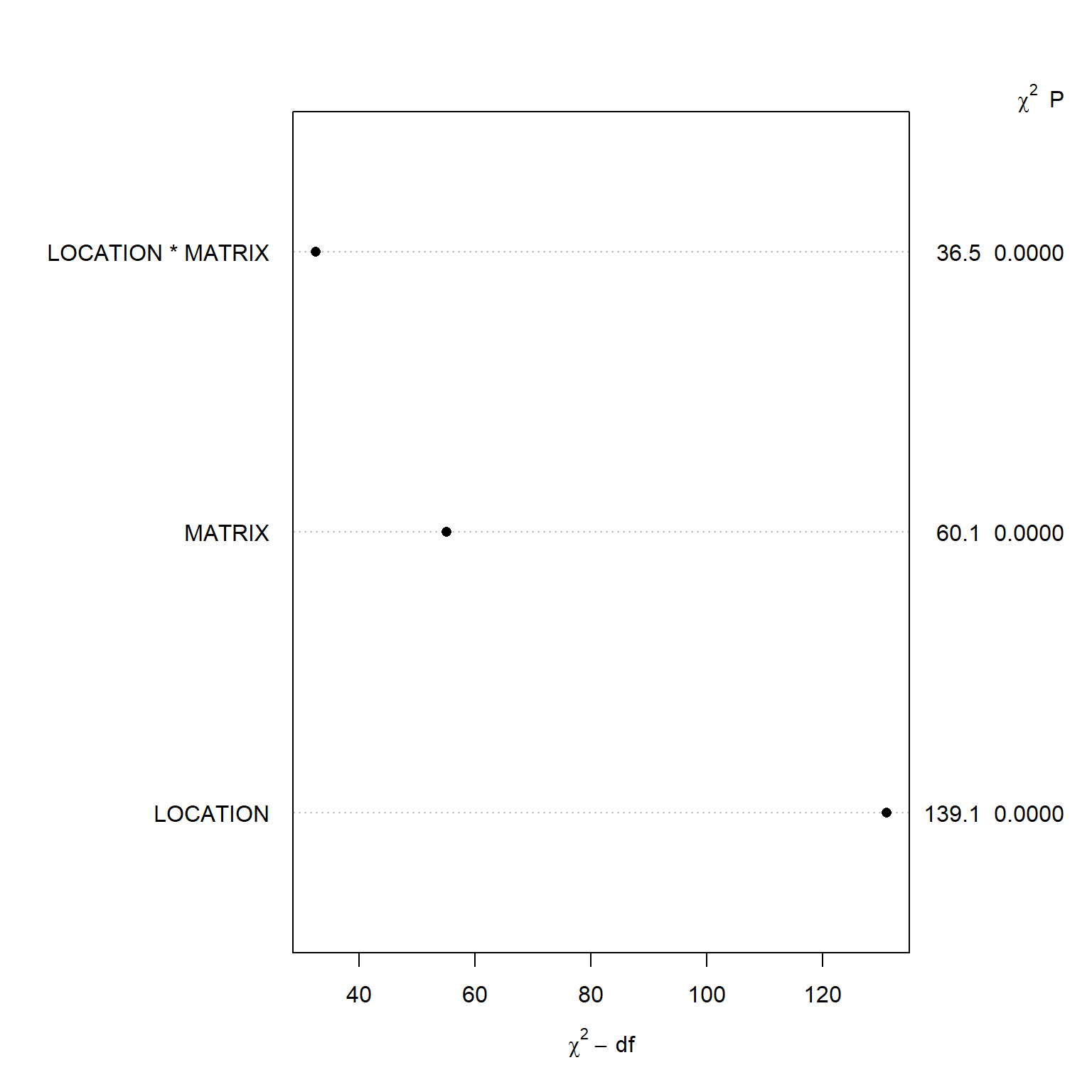
The Wald \(\chi^2\) statistic is 139 for LOCATION, 60.1 for MATRIX, and 36.5 for the interaction between depth and location (MATRIX:LOCATION). Let’s create a dot chart depicting the importance of variables in the model as measured by the Wald statistic and p-value.
plot(anova(f))
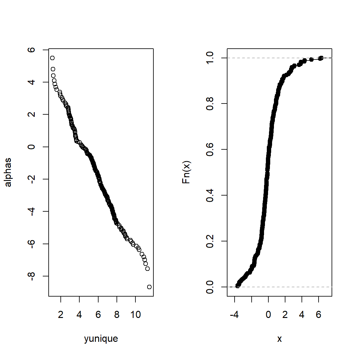
Let’s show the intercepts as a function of y to inspect the underlying conditional distribution. Let’s also inspect the distribution of residuals.
alphas <- coef(f)[1 : num.intercepts(f)]
yunique <- f$yunique[-1]
par(mfrow = c(1,2))
plot(yunique, alphas)
plot(ecdf(resid(ols(RESULT ~ LOCATION * MATRIX, data = d))), main = '')
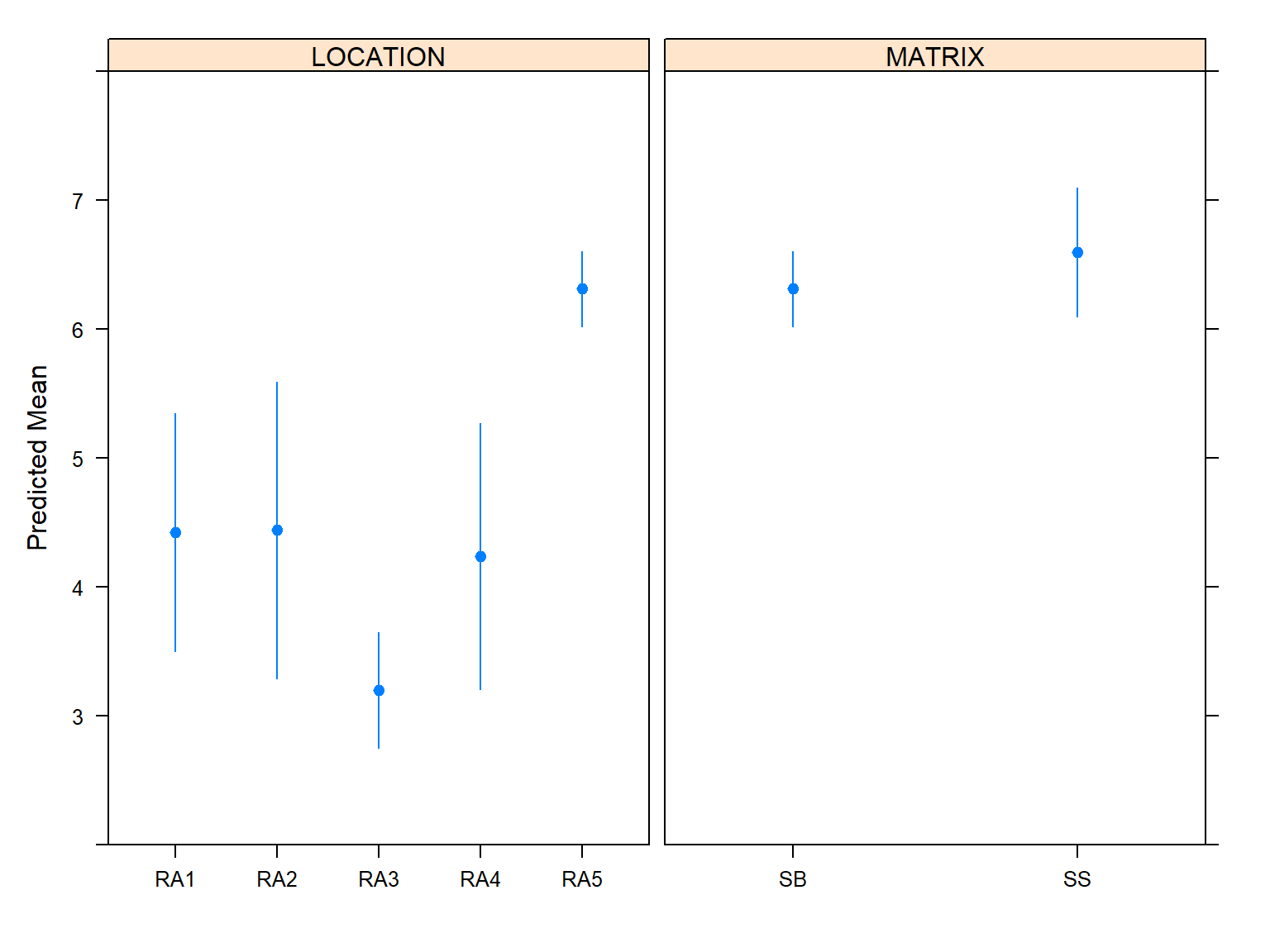
Whereas confidence intervals for means are approximate, the confidence intervals for odds ratios or exceedance probabilities are correct for ordinal models.
M <- Mean(f)
Predict(f, LOCATION, MATRIX, fun = M)
##    LOCATION MATRIX     yhat    lower    upper
## 1       RA1     SB 4.423752 3.498615 5.348890
## 2       RA2     SB 4.442087 3.292227 5.591948
## 3       RA3     SB 3.199625 2.752734 3.646516
## 4       RA4     SB 4.238769 3.205413 5.272125
## 5       RA5     SB 6.311153 6.020567 6.601740
## 6       RA1     SS 6.317480 5.741308 6.893652
## 7       RA2     SS 8.593215 7.988621 9.197809
## 8       RA3     SS 3.597675 3.108999 4.086350
## 9       RA4     SS 7.077969 6.426724 7.729214
## 10      RA5     SS 6.594971 6.093381 7.096561
##
## Response variable (y):
##
## Limits are 0.95 confidence limits
Let’s plot the predicted mean values.
plot(Predict(f, fun = M), ylab = 'Predicted Mean')
Let’s estimate the sample means with t-confidence limits.
with(d, summarize(RESULT, llist(LOCATION, MATRIX), smean.cl.normal))
##    LOCATION MATRIX   RESULT    Lower    Upper
## 1       RA1     SB 4.816087 3.514020 6.118154
## 2       RA1     SS 6.372400 5.724396 7.020404
## 3       RA2     SB 4.580909 2.680446 6.481373
## 4       RA2     SS 8.544000 7.943056 9.144944
## 5       RA3     SB 3.100000 2.849411 3.350589
## 6       RA3     SS 3.594800 3.175911 4.013689
## 7       RA4     SB 4.571429 1.759652 7.383205
## 8       RA4     SS 7.206800 6.364318 8.049282
## 9       RA5     SB 6.334933 6.187271 6.482596
## 10      RA5     SS 6.598000 6.269077 6.926923
Let’s compute the contrasts of the estimated regression coefficients obtained from the OLR model fit, along with standard errors, confidence limits, Z-statistics, and p-values.
contrast(
  f,
  list(
    LOCATION = c('RA1', 'RA2', 'RA3', 'RA4', 'RA5'),
    MATRIX = c('SS', 'SB')
  )
)
##      LOCATION MATRIX    Contrast      S.E.      Lower      Upper     Z Pr(>|z|)
##  1        RA1     SS  2.31648976 0.6997159  0.9450719  3.6879076  3.31   0.0009
##  2        RA2     SS  5.02211664 0.7236544  3.6037800  6.4404533  6.94   0.0000
##  3        RA3     SS -1.03589081 0.6556802 -2.3210004  0.2492188 -1.58   0.1141
##  4        RA4     SS  3.27049995 0.7314778  1.8368298  4.7041701  4.47   0.0000
##  5        RA5     SS  2.66690061 0.6810062  1.3321530  4.0016482  3.92   0.0001
##  6*       RA1     SB  0.00000000 0.0000000  0.0000000  0.0000000   NaN      NaN
##  7        RA2     SB  0.02214307 0.9108468 -1.7630838  1.8073700  0.02   0.9806
##  8        RA3     SB -1.57465875 0.6539419 -2.8563613 -0.2929562 -2.41   0.0160
##  9        RA4     SB -0.22479643 0.8628462 -1.9159440  1.4663511 -0.26   0.7945
## 10        RA5     SB  2.30849860 0.6249717  1.0835766  3.5334206  3.69   0.0002
##
## Redundant contrasts are denoted by *
##
## Confidence intervals are 0.95 individual intervals
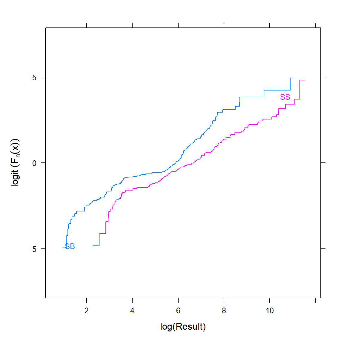
One of the assumptions underlying OLR is that the relationship between each pair of outcome groups is the same. In other words, OLR assumes that the coefficients that describe the relationship between, say, the lowest versus all higher categories of the response variable are the same as those that describe the relationship between the next lowest category and all higher categories. This is called the proportional odds assumption.
Let’s plot the logit transformation of the group-stratified empirical cumulative distribution functions for the response variable. First, let’s create the plot stratified by MATRIX using the Ecdf() function from the Hmisc R package.
Ecdf( ~ RESULT, group = MATRIX, data = d, fun = qlogis,
     xlab = 'log(Result)', ylab = expression(logit~(F[n](x))))
Now, let’s create the plot of the logit transformation of the empirical cumulative distribution functions stratified by LOCATION.
Ecdf( ~ RESULT, group = LOCATION, data = d, fun = qlogis,
     xlab = 'log(Result)', ylab = expression(logit~(F[n](x))))
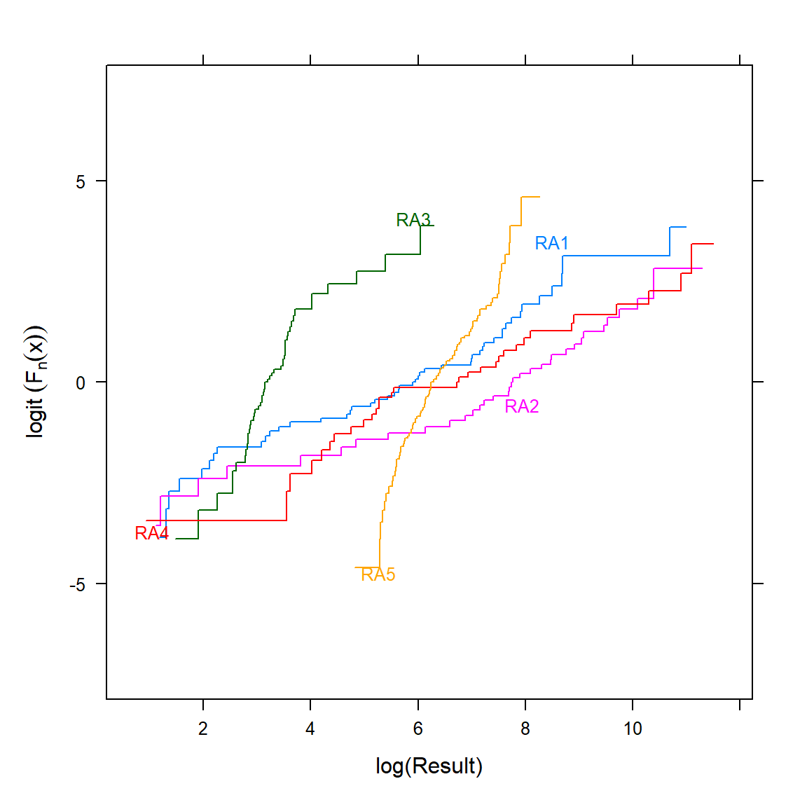
Non-parallelism is readily seen, indicating non-proportional odds. If PO doesn’t hold, an OLR model may still be better than the alternatives (note that the Wilcoxon and Kruskal-Wallis tests also assume PO to have optimal power). When PO does not hold, the odds ratio from the proportional odds model represents a kind of average odds ratio, and there is an almost one-to-one relationship between the odds ratio and the concordance probability, which is a simple translation of the Wilcoxon statistic (Harrell 2022c).
References
Harrell, F.E. 2015. Regression Modeling Strategies: With Applications to Linear Models, Logistic and Ordinal Regression, and Survival Analysis, 2nd Edition. Springer, Switzerland.
Harrell, F.E. 2022a. If You Like the Wilcoxon Test You Must Like the Proportional Odds Model. https://www.fharrell.com/post/wpo/. April.
Harrell, F.E. 2022b. Equivalence of Wilcoxon Statistic and Proportional Odds Model. https://www.fharrell.com/post/powilcoxon. April.
Harrell, F.E. 2022c. Violation of Proportional Odds is Not Fatal. https://www.fharrell.com/post/po/. April.
Liu, Q., B.E. Shepherd, C. Li, and F.E. Harrell. 2017. Modeling continuous response variables using ordinal regression. Stat Med. 36, 4316-4335.
- Posted on:
- April 17, 2022
- Length:
- 10 minute read, 1948 words
- See Also: