Rain Tomorrow Stacked Ensemble Model
By Charles Holbert
September 5, 2022
For this post, we will evaluate rainfall in Australia using daily weather observations from multiple Australian weather stations. The data include a target variable RainTomorrow, which identifies (Yes/No) whether there was rain on the following day. We will build a stacked ensemble machine learning model for use in predicting if there will be rain tomorrow. Ensemble machine learning methods use multiple learning algorithms to obtain better predictive performance than could be obtained from any individual learning algorithm.
Load Libraries
Load libraries required to analyze the data.
# Load libraries
library(dplyr)
library(tidyr)
library(ggplot2)
library(scales)
library(rsample)
Read Data
Load the data from the csv file and inspect data structure. This dataset contains over 140,000 daily observations from over 45 Australian weather stations. RainTomorrow is the target variable to predict. If this column is Yes, rain for the next day was 1 mm or more.
# Read data in comma-delimited file
dat <- read.csv('data/weatherAUS.csv', header = T)

# Read location data in comma-delimited file
locs <- read.csv('data/locations.csv', header = T)

# Inspect structure of data
str(dat)
## 'data.frame':	145460 obs. of  23 variables:
##  $ Date         : chr  "2008-12-01" "2008-12-02" "2008-12-03" "2008-12-04" ...
##  $ Location     : chr  "Albury" "Albury" "Albury" "Albury" ...
##  $ MinTemp      : num  13.4 7.4 12.9 9.2 17.5 14.6 14.3 7.7 9.7 13.1 ...
##  $ MaxTemp      : num  22.9 25.1 25.7 28 32.3 29.7 25 26.7 31.9 30.1 ...
##  $ Rainfall     : num  0.6 0 0 0 1 0.2 0 0 0 1.4 ...
##  $ Evaporation  : num  NA NA NA NA NA NA NA NA NA NA ...
##  $ Sunshine     : num  NA NA NA NA NA NA NA NA NA NA ...
##  $ WindGustDir  : chr  "W" "WNW" "WSW" "NE" ...
##  $ WindGustSpeed: int  44 44 46 24 41 56 50 35 80 28 ...
##  $ WindDir9am   : chr  "W" "NNW" "W" "SE" ...
##  $ WindDir3pm   : chr  "WNW" "WSW" "WSW" "E" ...
##  $ WindSpeed9am : int  20 4 19 11 7 19 20 6 7 15 ...
##  $ WindSpeed3pm : int  24 22 26 9 20 24 24 17 28 11 ...
##  $ Humidity9am  : int  71 44 38 45 82 55 49 48 42 58 ...
##  $ Humidity3pm  : int  22 25 30 16 33 23 19 19 9 27 ...
##  $ Pressure9am  : num  1008 1011 1008 1018 1011 ...
##  $ Pressure3pm  : num  1007 1008 1009 1013 1006 ...
##  $ Cloud9am     : int  8 NA NA NA 7 NA 1 NA NA NA ...
##  $ Cloud3pm     : int  NA NA 2 NA 8 NA NA NA NA NA ...
##  $ Temp9am      : num  16.9 17.2 21 18.1 17.8 20.6 18.1 16.3 18.3 20.1 ...
##  $ Temp3pm      : num  21.8 24.3 23.2 26.5 29.7 28.9 24.6 25.5 30.2 28.2 ...
##  $ RainToday    : chr  "No" "No" "No" "No" ...
##  $ RainTomorrow : chr  "No" "No" "No" "No" ...
Prep Data
Let’s prep the data prior to modeling. First, we will join the data with a locations file that contains geographical coordinates and an assigned climate zone for each weather station. Locations with approximately similar climates have been combined into eight climate zones, which include the following:
- Climate zone 1 - high humidity summer, warm winter
- Climate zone 2 - warm humid summer, mild winter
- Climate zone 3 - hot dry summer, warm winter
- Climate zone 4 - hot dry summer, cool winter
- Climate zone 5 - warm temperate
- Climate zone 6 - mild temperate
- Climate zone 7 - cool temperate
- Climate zone 8 - alpine
Let’s also add some additional variables to the data, including month, year, and differential humidity, temperature, and pressure.
# Prep the data
dat <- dat %>%
  left_join(locs, by = 'Location') %>%
  mutate(
    Date = as.Date(dat$Date),
    Zone = as.factor(Zone),
    Month = lubridate::month(Date, label = TRUE),
    Year = as.factor(lubridate::year(Date)),
    diffHumidity = Humidity3pm - Humidity9am,
    diffTemp = Temp3pm - Temp9am,
    diffPressure = Pressure3pm - Pressure9am
  )
Finalize Data
Finally, let’s select the variables that will be used in the model.
# Select final variables
dat <- dat %>%
  dplyr::select(
    RainTomorrow,
    RainToday,
    Zone,
    Month,
    Sunshine,
    diffTemp,
    diffPressure,
    diffHumidity,
    WindGustSpeed,
    MaxTemp,
    Temp3pm ,
    Rainfall,
    Humidity9am,
    Humidity3pm,
    Pressure9am,
    Pressure3pm
  ) %>%
  tidyr::drop_na() %>%
  droplevels() %>%
  mutate_if(is.character, as.factor) %>%
  mutate(across(Sunshine:Pressure3pm, scales::rescale)) %>%
  mutate(
    Month = factor(Month, ordered = FALSE),
    RainTomorrow = relevel(RainTomorrow, ref = 'Yes')
  )

# Check structure of final data
str(dat)
## 'data.frame':	69124 obs. of  16 variables:
##  $ RainTomorrow : Factor w/ 2 levels "Yes","No": 2 2 2 2 2 2 2 2 2 2 ...
##  $ RainToday    : Factor w/ 2 levels "No","Yes": 1 1 1 1 1 1 1 1 1 1 ...
##  $ Zone         : Factor w/ 7 levels "1","2","3","4",..: 4 4 4 4 4 4 4 4 4 4 ...
##  $ Month        : Factor w/ 12 levels "Jan","Feb","Mar",..: 1 1 1 1 1 1 1 1 1 1 ...
##  $ Sunshine     : num  0.848 0.897 0.731 0.841 0.579 ...
##  $ diffTemp     : num  0.538 0.536 0.521 0.53 0.459 ...
##  $ diffPressure : num  0.51 0.552 0.463 0.444 0.456 ...
##  $ diffHumidity : num  0.462 0.379 0.39 0.418 0.478 ...
##  $ WindGustSpeed: num  0.333 0.239 0.316 0.188 0.222 ...
##  $ MaxTemp      : num  0.707 0.564 0.761 0.78 0.839 ...
##  $ Temp3pm      : num  0.7 0.55 0.736 0.752 0.8 ...
##  $ Rainfall     : num  0 0 0 0 0 0 0 0 0 0 ...
##  $ Humidity9am  : num  0.2 0.3 0.42 0.37 0.19 0.26 0.33 0.25 0.46 0.61 ...
##  $ Humidity3pm  : num  0.13 0.08 0.22 0.22 0.15 0.19 0.15 0.09 0.28 0.14 ...
##  $ Pressure9am  : num  0.431 0.541 0.531 0.538 0.504 ...
##  $ Pressure3pm  : num  0.442 0.566 0.519 0.518 0.49 ...
Split Data
Let’s split the data into training and testing data sets within the stratification variable RainTomorrow. This helps ensure that the splits have equivalent proportions as the original data.
# Split data in training and testing sets
set.seed(123)

dat_split <- rsample::initial_split(dat, prop = 0.75, strata = RainTomorrow)
dat_train <- rsample::training(dat_split)
dat_test <- rsample::testing(dat_split)
dat_split
## <Training/Testing/Total>
## <51842/17282/69124>
Train Model
Let’s train a stacked ensemble machine learning model for predicting rain tomorrow. Ensembling is the process of combining predictions from multiple models to form a more accurate model. Because individual algorithms have unique strengths, ensembles combine their strengths to produce a better model. For our model, let’s use three base learners that are called by a super learner to make a final prediction based on the predictions of the base learners. The base learners will consist of a generalized linear model (GLM), a random forest (RF) model, and a gradient boosting machine (GBM) model with 5-fold cross-validation.
Let’s use the H2O machine learning platform. H2O is an in-memory platform for distributed, scalable machine learning. The R interface for H2O offers parallelized implementations of many supervised and unsupervised machine learning algorithms.
Start H2O cluster
To use H2O you have to imagine that all the work is being done on a remote server you are communicating with. Let’s load the library and then initialize the server.
# Load libraries
library(h2o)

# Connect to H2O
h2o.no_progress()   # turn off progress bars for brevity
h2o.init(min_mem_size = '10G', max_mem_size= '100G')   # connect to H2O instance
##
## H2O is not running yet, starting it now...
##
## Note:  In case of errors look at the following log files:
##     C:\Users\cholbert\AppData\Local\Temp\RtmpsHWS7o\file62a014d23829/h2o_cholbert_started_from_r.out
##     C:\Users\cholbert\AppData\Local\Temp\RtmpsHWS7o\file62a0319b1eea/h2o_cholbert_started_from_r.err
##
##
## Starting H2O JVM and connecting: . Connection successful!
##
## R is connected to the H2O cluster:
##     H2O cluster uptime:         11 seconds 506 milliseconds
##     H2O cluster timezone:       America/Denver
##     H2O data parsing timezone:  UTC
##     H2O cluster version:        3.36.1.2
##     H2O cluster version age:    3 months and 12 days !!!
##     H2O cluster name:           H2O_started_from_R_cholbert_elp849
##     H2O cluster total nodes:    1
##     H2O cluster total memory:   88.78 GB
##     H2O cluster total cores:    8
##     H2O cluster allowed cores:  8
##     H2O cluster healthy:        TRUE
##     H2O Connection ip:          localhost
##     H2O Connection port:        54321
##     H2O Connection proxy:       NA
##     H2O Internal Security:      FALSE
##     R Version:                  R version 4.2.1 (2022-06-23 ucrt)
#h2o.init(max_mem_size = '200G')   # connect to H2O instance
H2O data frames
Let’s import the rain tomorrow data into the local H2O cluster. The H2O frame is the main data structure used on the H2O cluster for data manipulation and modelling. Let’s also get the names of the response and features.
# Create h20 dataframe
train_h2o <- dat_train %>% as.h2o()
test_h2o <- dat_test %>% as.h2o()

# Get names of response and features
myvars <- names(dat)
Y <- 'RainTomorrow'
X <- setdiff(myvars, Y)
GLM Model
The first classification algorithm we will train and evaluate is logistic regression.
# Train & cross-validate a GLM model
best_glm <- h2o.glm(
  x = X, y = Y, training_frame = train_h2o,
  alpha = 0.1,
  remove_collinear_columns = TRUE,
  nfolds = 5, fold_assignment = 'Modulo',
  keep_cross_validation_predictions = TRUE,
  seed = 123
)
Random Forest Model
The second classification algorithm we will train and evaluate is RF.
# Train & cross-validate a RF model
best_rf <- h2o.randomForest(
  x = X, y = Y, training_frame = train_h2o,
  ntrees = 500,
  mtries = 8,
  max_depth = 30, min_rows = 1,
  sample_rate = 0.8,
  nfolds = 5, fold_assignment = 'Modulo',
  keep_cross_validation_predictions = TRUE,
  seed = 123,
  stopping_rounds = 50, stopping_metric = 'AUC',
  stopping_tolerance = 0
)
GBM Model
The third classification algorithm we will train and evaluate is GBM.
# Train & cross-validate a GBM model
best_gbm <- h2o.gbm(
  x = X, y = Y, training_frame = train_h2o,
  ntrees = 500,
  learn_rate = 0.01,
  max_depth = 7, min_rows = 5,
  sample_rate = 0.8,
  nfolds = 5, fold_assignment = 'Modulo',
  keep_cross_validation_predictions = TRUE,
  seed = 123,
  stopping_rounds = 50, stopping_metric = 'AUC',
  stopping_tolerance = 0
)
Stacked Ensemble Model
Now, let’s train a stacked tree ensemble.
# Train a stacked tree ensemble
ensemble_tree <- h2o.stackedEnsemble(
  x = X, y = Y, training_frame = train_h2o,
  model_id = 'my_tree_ensemble',
  base_models = list(best_glm, best_rf, best_gbm),
  metalearner_algorithm = 'drf'
)

print(ensemble_tree)
## Model Details:
## ==============
##
## H2OBinomialModel: stackedensemble
## Model ID:  my_tree_ensemble
## Number of Base Models: 3
##
## Base Models (count by algorithm type):
##
## drf gbm glm
##   1   1   1
##
## Metalearner:
##
## Metalearner algorithm: drf
## Metalearner hyperparameters:
##
##
## H2OBinomialMetrics: stackedensemble
## ** Reported on training data. **
##
## MSE:  0.02534384
## RMSE:  0.1591975
## LogLoss:  0.1155514
## Mean Per-Class Error:  0.008285078
## AUC:  0.9997194
## AUCPR:  0.9990411
## Gini:  0.9994387
##
## Confusion Matrix (vertical: actual; across: predicted) for F1-optimal threshold:
##          No  Yes    Error      Rate
## No     7630   48 0.006252  =48/7678
## Yes      23 2206 0.010319  =23/2229
## Totals 7653 2254 0.007167  =71/9907
##
## Maximum Metrics: Maximum metrics at their respective thresholds
##                         metric threshold       value idx
## 1                       max f1  0.443340    0.984162 164
## 2                       max f2  0.422879    0.989374 168
## 3                 max f0point5  0.513444    0.988688 146
## 4                 max accuracy  0.476957    0.992833 156
## 5                max precision  0.999963    1.000000   0
## 6                   max recall  0.315015    1.000000 195
## 7              max specificity  0.999963    1.000000   0
## 8             max absolute_mcc  0.443340    0.979557 164
## 9   max min_per_class_accuracy  0.430000    0.991534 167
## 10 max mean_per_class_accuracy  0.422879    0.992721 168
## 11                     max tns  0.999963 7678.000000   0
## 12                     max fns  0.999963 2099.000000   0
## 13                     max fps  0.000074 7678.000000 399
## 14                     max tps  0.315015 2229.000000 195
## 15                     max tnr  0.999963    1.000000   0
## 16                     max fnr  0.999963    0.941678   0
## 17                     max fpr  0.000074    1.000000 399
## 18                     max tpr  0.315015    1.000000 195
##
## Gains/Lift Table: Extract with `h2o.gainsLift(<model>, <data>)` or `h2o.gainsLift(<model>, valid=<T/F>, xval=<T/F>)`
Model Performance on Training Data
Obtain performance metrics of the ensemble model on the training data.
# Generate a ModelMetrics object for training data
perf_train <- h2o.performance(ensemble_tree, train_h2o)
perf_train
## H2OBinomialMetrics: stackedensemble
##
## MSE:  0.02524074
## RMSE:  0.1588733
## LogLoss:  0.1148666
## Mean Per-Class Error:  0.008935706
## AUC:  0.9997393
## AUCPR:  0.9990858
## Gini:  0.9994785
##
## Confusion Matrix (vertical: actual; across: predicted) for F1-optimal threshold:
##           No   Yes    Error        Rate
## No     40217   209 0.005170  =209/40426
## Yes      145 11271 0.012701  =145/11416
## Totals 40362 11480 0.006828  =354/51842
##
## Maximum Metrics: Maximum metrics at their respective thresholds
##                         metric threshold        value idx
## 1                       max f1  0.443879     0.984539 167
## 2                       max f2  0.405221     0.989239 176
## 3                 max f0point5  0.514519     0.988433 149
## 4                 max accuracy  0.463629     0.993172 162
## 5                max precision  0.999949     1.000000   0
## 6                   max recall  0.245582     1.000000 225
## 7              max specificity  0.999949     1.000000   0
## 8             max absolute_mcc  0.443879     0.980163 167
## 9   max min_per_class_accuracy  0.423013     0.992379 172
## 10 max mean_per_class_accuracy  0.405221     0.992663 176
## 11                     max tns  0.999949 40426.000000   0
## 12                     max fns  0.999949 10780.000000   0
## 13                     max fps  0.000087 40426.000000 399
## 14                     max tps  0.245582 11416.000000 225
## 15                     max tnr  0.999949     1.000000   0
## 16                     max fnr  0.999949     0.944289   0
## 17                     max fpr  0.000087     1.000000 399
## 18                     max tpr  0.245582     1.000000 225
##
## Gains/Lift Table: Extract with `h2o.gainsLift(<model>, <data>)` or `h2o.gainsLift(<model>, valid=<T/F>, xval=<T/F>)`
Obtain just the confusion matrix on the training data.
h2o.confusionMatrix(perf_train)
## Confusion Matrix (vertical: actual; across: predicted)  for max f1 @ threshold = 0.443879086348143:
##           No   Yes    Error        Rate
## No     40217   209 0.005170  =209/40426
## Yes      145 11271 0.012701  =145/11416
## Totals 40362 11480 0.006828  =354/51842
Create ROC curve for the training data.
# Plot ROC curve for training data
fpr <- (perf_train@metrics$thresholds_and_metric_scores$fpr)
tpr <- (perf_train@metrics$thresholds_and_metric_scores$tpr)
plot(fpr, tpr, type = 'l', col = 'blue')
abline(0, 1)
title('AUC Training Data')
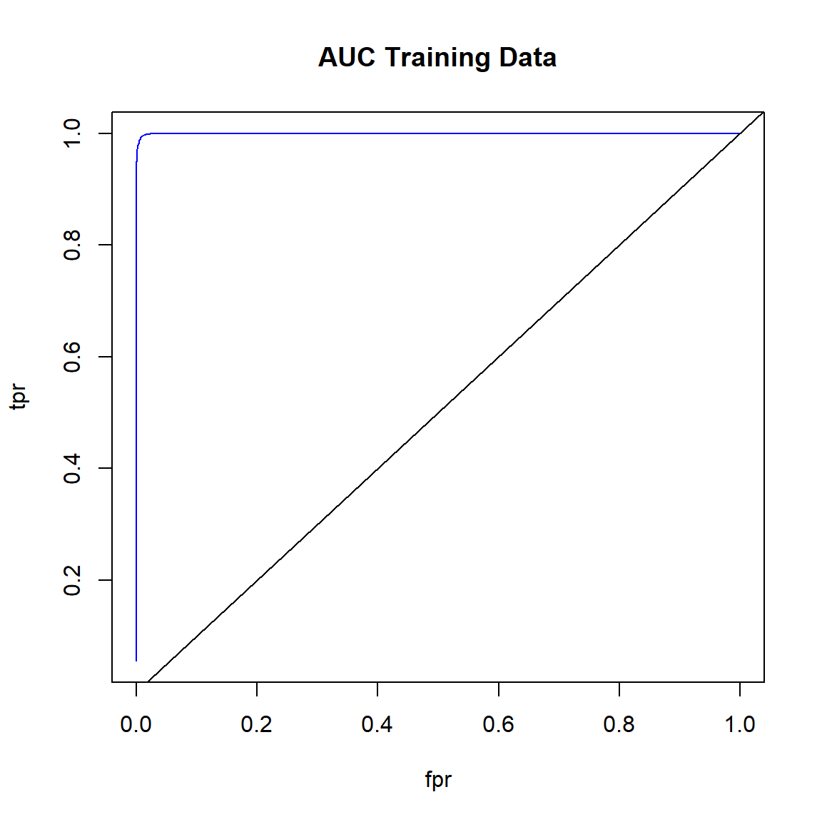
Get the area under the ROC curve for the training data.
# Area under the ROC curve (AUC) on training data
h2o.auc(perf_train)
## [1] 0.9997393
Model Performance on Test Data
Obtain performance metrics of the ensemble model on the test data.
# Generate a ModelMetrics object for test data
perf_test <- h2o.performance(ensemble_tree, test_h2o)
perf_test
## H2OBinomialMetrics: stackedensemble
##
## MSE:  0.1011505
## RMSE:  0.3180416
## LogLoss:  0.3380491
## Mean Per-Class Error:  0.2119058
## AUC:  0.8928204
## AUCPR:  0.7395507
## Gini:  0.7856408
##
## Confusion Matrix (vertical: actual; across: predicted) for F1-optimal threshold:
##           No  Yes    Error         Rate
## No     12180 1296 0.096171  =1296/13476
## Yes     1247 2559 0.327641   =1247/3806
## Totals 13427 3855 0.147147  =2543/17282
##
## Maximum Metrics: Maximum metrics at their respective thresholds
##                         metric threshold        value idx
## 1                       max f1  0.396894     0.668059 193
## 2                       max f2  0.113106     0.754371 317
## 3                 max f0point5  0.586395     0.703334 130
## 4                 max accuracy  0.532112     0.860664 147
## 5                max precision  0.999934     0.987234   0
## 6                   max recall  0.000132     1.000000 399
## 7              max specificity  0.999934     0.999777   0
## 8             max absolute_mcc  0.413406     0.574857 188
## 9   max min_per_class_accuracy  0.224521     0.807147 261
## 10 max mean_per_class_accuracy  0.206603     0.808660 269
## 11                     max tns  0.999934 13473.000000   0
## 12                     max fns  0.999934  3574.000000   0
## 13                     max fps  0.000132 13476.000000 399
## 14                     max tps  0.000132  3806.000000 399
## 15                     max tnr  0.999934     0.999777   0
## 16                     max fnr  0.999934     0.939044   0
## 17                     max fpr  0.000132     1.000000 399
## 18                     max tpr  0.000132     1.000000 399
##
## Gains/Lift Table: Extract with `h2o.gainsLift(<model>, <data>)` or `h2o.gainsLift(<model>, valid=<T/F>, xval=<T/F>)`
Obtain just the confusion matrix on the training data.
h2o.confusionMatrix(perf_test)
## Confusion Matrix (vertical: actual; across: predicted)  for max f1 @ threshold = 0.396893655508757:
##           No  Yes    Error         Rate
## No     12180 1296 0.096171  =1296/13476
## Yes     1247 2559 0.327641   =1247/3806
## Totals 13427 3855 0.147147  =2543/17282
Create ROC curve for the test data.
# Plot ROC curve for test data
fpr <- (perf_test@metrics$thresholds_and_metric_scores$fpr)
tpr <- (perf_test@metrics$thresholds_and_metric_scores$tpr)
plot(fpr, tpr, type = 'l', col = 'blue')
abline(0, 1)
title('AUC Test Data')
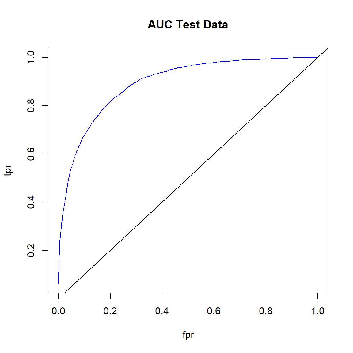
Get the area under the ROC curve for the test data.
# Area under the ROC curve (AUC) on test data
h2o.auc(perf_test)
## [1] 0.8928204
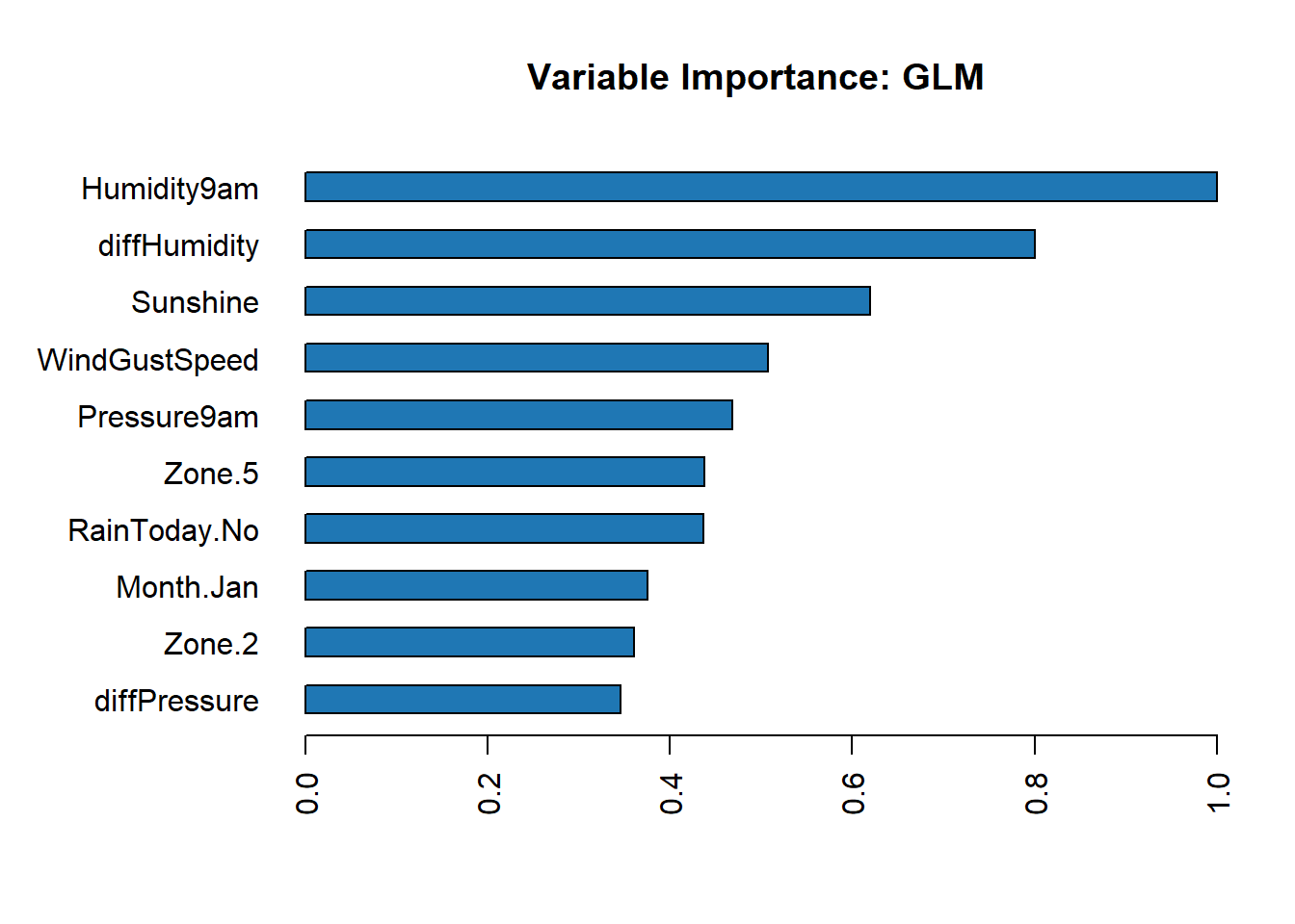
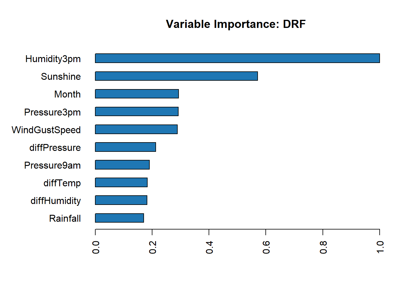
Feature Importance
Individual Models
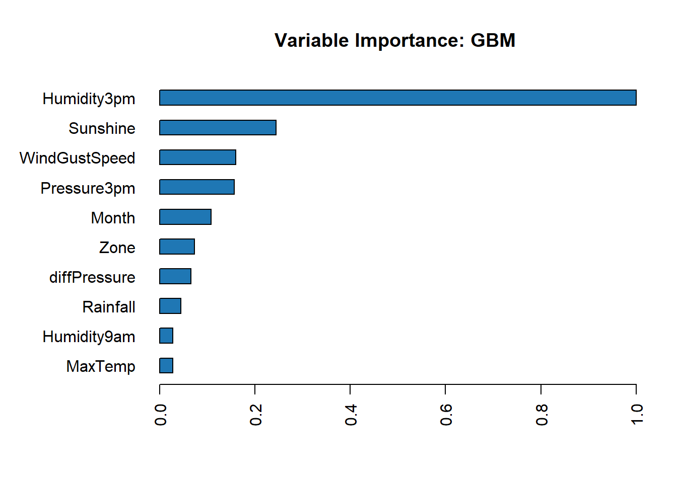
Get the feature importance for each individual model.
# Feature importance for each individual model
h2o.varimp_plot(best_glm)
h2o.varimp_plot(best_rf)
h2o.varimp_plot(best_gbm)
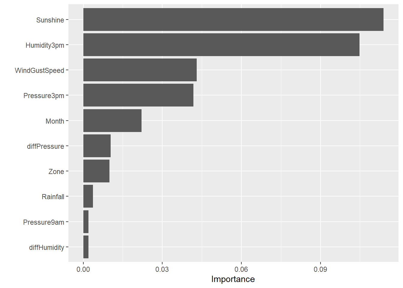
Ensemble Model
Get the permutation-based feature importance for the stacked ensemble model.
library(vip)
set.seed(123)

# Create prediction wrapper function
pred_fun <- function(object, newdata)  {
  results <- as.vector(h2o.predict(object, as.h2o(newdata))$Yes)
  return(results)
}

# Get feature importance
vip(
  ensemble_tree,
  train = as.data.frame(train_h2o),
  method = 'permute',
  target = 'RainTomorrow',
  reference_class = 'Yes',
  metric = 'auc',
  nsim = 5,
  sample_frac = 0.5,
  pred_wrapper = pred_fun
)
Shut down the H2O cluster
# Shut down the H2O cluster
h2o.shutdown(prompt = FALSE)
- Posted on:
- September 5, 2022
- Length:
- 13 minute read, 2743 words
- See Also: