Shaded Relief Basemap Using rayshader

By Charles Holbert

September 6, 2022

Shaded relief of surface elevation illustrates the shape of the terrain in a realistic fashion by showing how the three-dimensional surface would be illuminated from a point light source. Generally, shaded relief is intended for use as a basemap layer that is added to other maps. It conveys an immediate and direct impression of a landscape and can be much easier to understand than two-dimensional maps. Unfortunately, the R package ggplot2 does not support multiple color and fill scales. This limits using shaded relief as a baselayer when using ggplot2 to create maps of other data requiring a fill scale.

This post illustrates the use of the rayshader R library for creating a shaded relief basemap using ggplot2. The rayshader library uses elevation data in a base R matrix and a combination of raytracing, hillshading algorithms, and overlays to generate 2D and 3D maps.

Load Libraries

Let’s load the libraries and custom functions that will be used to download, process, and plot the data.

# Load libraries
library(dplyr)
library(ggplot2)
library(tigris)
library(sf)
library(raster)
library(RStoolbox)
library(ggsflabel)
library(rayshader)

source('functions/array_to_RasterStack.R')

Plot Theme

The R package ggplot2 is remarkably extensible and customizable both through specific graphical components (geom_, scale_, aes, etc) or by theme components (grid lines, background colors, fonts, etc). Additionally, there are fully established themes that change many theme components at once. For efficiency, let’s create a ggplot2 custom theme for our maps.

# Define ggplot function
theme_gppr <- function(){ 
    
    theme_void() %+replace%    # replace elements we want to change
    
    theme(
      plot.title = element_text(
                   margin = margin(b = 2),
                   size = 14,
                   color = 'black',
                   face = 'bold',
                   hjust = 0),
      
      plot.subtitle = element_text(
                   margin = margin(b = 2),
                   size = 12,
                   color = 'black',
                   face = 'italic',
                   hjust = 0),
      
      plot.caption = element_text(hjust = 0, size = 8),
      
      legend.position = 'right',
      legend.title = element_text(size = 9),
      legend.text = element_text(size = 9),
      
      plot.margin = unit(c(0.1, 0.0, 0.2, 0.0), "in")
    )
}

Load Data

Previously downloaded data include shapefiles for the State of Utah School and Institutional Trust Lands Administration (SITLA) surface land ownership data and major Utah water bodies.

# Load waterbodies shapefile
water <- sf::st_read('shapes/utah_water.shp', quiet = T)

# Load land ownership shapefile
lands <- sf::st_read('shapes/UT_SITLA_Ownership_LandOwnership.shp', quiet = T)

A shapefile for Utah counties can be downloaded using the R package tigris. The tigris package allows users to directly download and use TIGER/Line shapefiles from the US Census Bureau.

# Get Utah counties using tigris
utah_counties <- counties(
  state = 'Utah', cb = TRUE,
  resolution = '20m', progress_bar = FALSE)

The R package elevatr can be used for accessing elevation data from from the AWS Open Data Terrain Tiles and the Open Topography Global datasets API for raster DEMs. For point elevation data, the USGS Elevation Point Query Service may be used or the point elevations may be derived from the AWS Tiles.

# Use elevatr to get elevation data
elev <- elevatr::get_elev_raster(
  locations = utah_counties$geometry, z = 7, clip = 'locations'
)

Surface Color Map

Let’s use the sphere_shade() function to calculate a color map using the surface normals and hemispherical UV mapping. The sphere_shade() function maps an RGB texture to a hillshade by spherical mapping.

# Convert elevation raster to matrix
elmat <- raster_to_matrix(elev)

# Calculate a color for each point on the surface using the surface normals and
# hemispherical UV mapping.
sunshade <- elmat %>%
  sphere_shade(sunangle = 315, texture = 'bw')

Now, let’s convert the surface color map to a raster and assign dimensions and projection using the original elevation raster file.

# Convert sunshade to raster
dd <- array_to_RasterStack(
  sunshade,
  type = 'stack',
  alpha_mask = TRUE,
  return_alpha = FALSE
)

# Assign dimensions
dd@extent@xmin <- elev@extent@xmin
dd@extent@xmax <- elev@extent@xmax
dd@extent@ymin <- elev@extent@ymin
dd@extent@ymax <- elev@extent@ymax

# Assign projection
crs(dd) <- crs(elev)

Maps

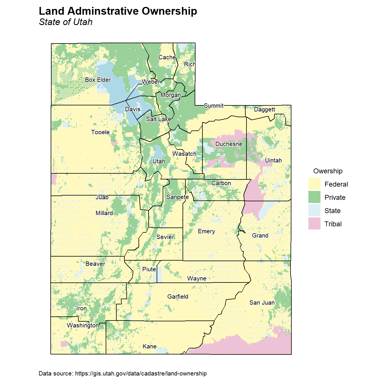
Land Ownership

Let’s create a map showing land ownership using the SITLA land ownership data. This statewide dataset is a compilation of all surface land ownership administration and designation categories. Both the SITLA and the Bureau of Land Management (BLM) update this dataset regularly.

# Land ownership map
cols <- c('#FFF062', 'green4', 'lightblue', '#D26799')
ggplot() +
  geom_sf(data = lands, aes(fill = OWNER), color = NA) +
  geom_sf(data = water, color = NA, fill = 'lightblue', size = 0.6, alpha = 1) +
  geom_sf(data = utah_counties, color = 'black', fill = NA) +
  geom_sf_text_repel(data = utah_counties, aes(label = NAME),
                     size = 2.8, bg.color = 'white', color = 'black') +
  coord_sf(datum = sf::st_crs(utah_counties)) +
  scale_fill_manual(values = alpha(cols, 0.4)) +
  labs(title = 'Land Adminstrative Ownership',
       subtitle = 'State of Utah',
       caption = 'Data source: https://gis.utah.gov/data/cadastre/land-ownership',
       fill = 'Owership') +
  theme_gppr()

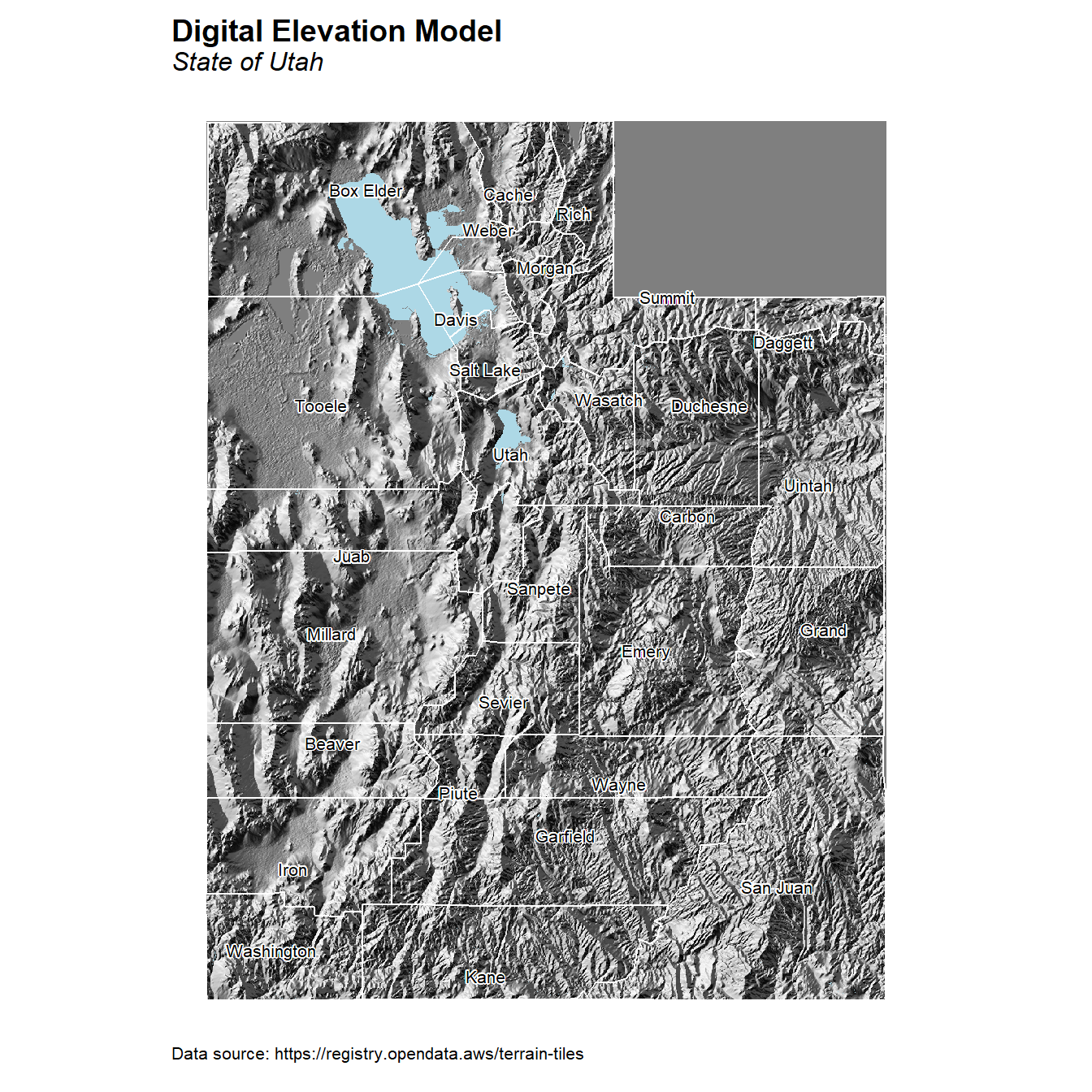
Shaded Relief Map

Let’s create a shaded relief map using rayshader() and the digital elevation data downloaded from the AWS Tiles.

# Elevation map
ggRGB(dd, r = 1, g = 2, b = 3, maxpixels = 5e+08) +
  geom_sf(data = water, color = NA, fill = 'lightblue', size = 0.6, alpha = 1) +
  geom_sf(data = utah_counties, color = 'white', fill = NA) +
  geom_sf_text_repel(data = utah_counties, aes(label = NAME),
                     size = 2.8, bg.color = 'white', color = 'black') +
  coord_sf(datum = sf::st_crs(utah_counties)) +
  labs(title = 'Digital Elevation Model',
       subtitle = 'State of Utah',
       caption = 'Data source: https://registry.opendata.aws/terrain-tiles',
       fill = 'Owership') +
  theme_gppr()

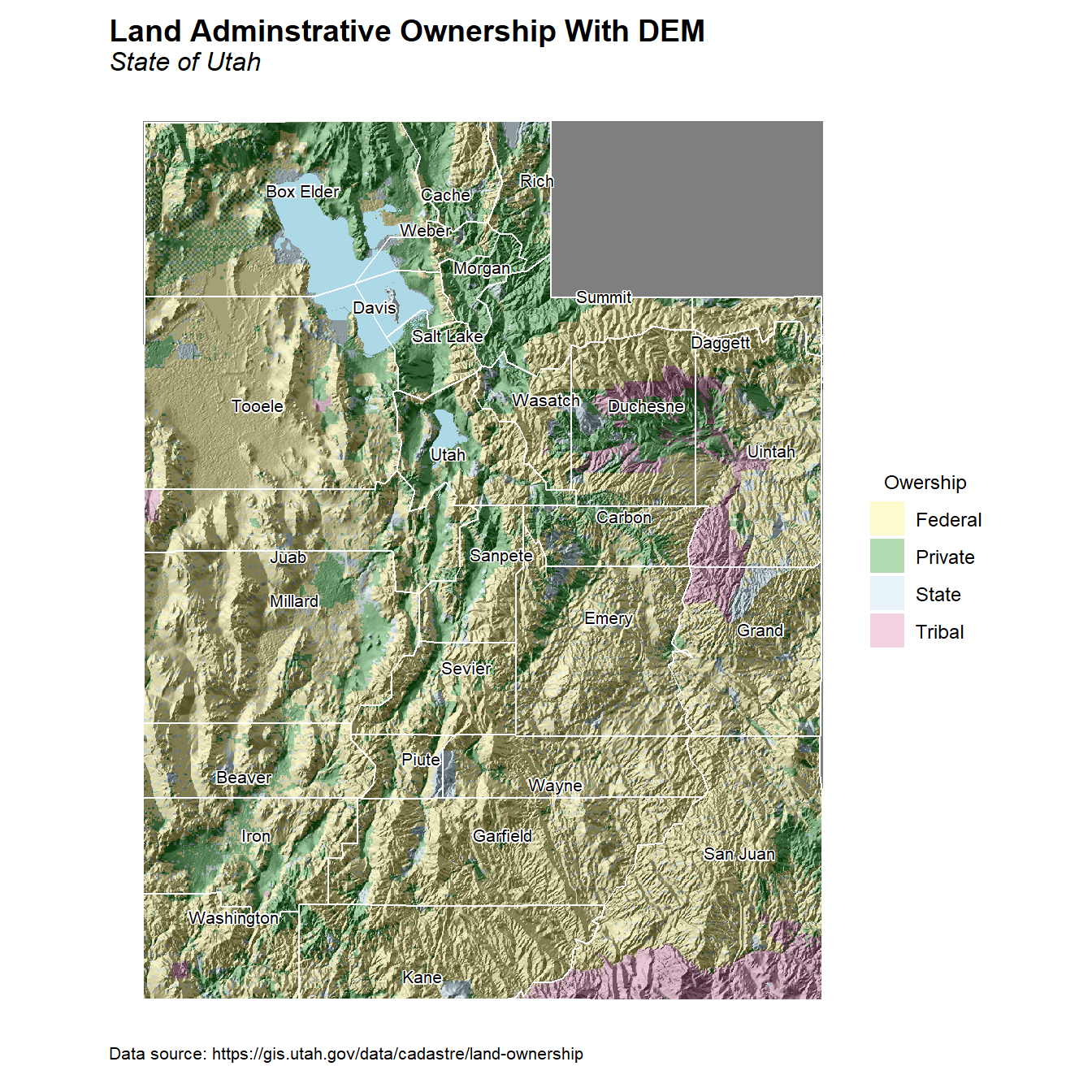
Land Ownership With Shaded Relief Map

Now, let’s create a map showing land ownership using shaded relief as a basemap.

# Combined map
ggRGB(dd, r = 1, g = 2, b = 3, maxpixels = 5e+08) +
  geom_sf(data = lands, aes(fill = OWNER), color = NA) +
  geom_sf(data = water, color = NA, fill = 'lightblue', size = 0.6, alpha = 1) +
  geom_sf(data = utah_counties, color = 'white', fill = NA) +
  geom_sf_text_repel(data = utah_counties, aes(label = NAME),
                     size = 2.8, bg.color = 'white', color = 'black') +
  coord_sf(datum = sf::st_crs(utah_counties)) +
  scale_fill_manual(values = alpha(cols, 0.3)) +
  labs(title = 'Land Adminstrative Ownership With DEM',
       subtitle = 'State of Utah',
       caption = 'Data source: https://gis.utah.gov/data/cadastre/land-ownership',
       fill = 'Owership') +
  theme_gppr()

Final Thoughts

The rayshader library enables users to create 2D and 3D visualizations using elevation data. This post demonstrates how output from rayshader can be used within existing work products that rely on ggplot2. We’ve downloaded digital elevation data, converted it to the needed format, created a surface relief map, rendered a high-quality 2D image, and then annotated it to create a final map.

Posted on:: September 6, 2022

Length:: 5 minute read, 1049 words

See Also: