Shaded Relief Basemap Using ggplot2
By Charles Holbert
July 25, 2022
Shaded relief of surface elevation illustrates the shape of the terrain in a realistic fashion by showing how the three-dimensional surface would be illuminated from a point light source. Generally, shaded relief is intended for use as a basemap layer that is added to other maps. It conveys an immediate and direct impression of a landscape and can be much easier to understand than two-dimensional maps. Unfortunately, the R package ggplot2 does not support multiple color and fill scales. This limits using shaded relief as a baselayer when using ggplot2 to create maps of other data requiring a fill scale.
This post illustrates the use of geom_relief(), a new aesthetic mapping layer, or geom (geometric object), for creating a shaded relief basemap using ggplot2.
Load Libraries
In R, the fundamental unit of reproducible code is the package, also referred to as a library. A package bundles together code, data, and documentation into a well-defined format that is easy to share with others. Let’s load the libraries that will be used to download, process, and plot the data.
# Load libraries
library(dplyr)
library(ggplot2)
library(tigris)
library(sf)
library(raster)
library(ggsflabel)
library(data.table)
Shaded Relief Map Function
Analytical shaded relief generated from Digital Elevation Models (DEMs) takes the form of raster image files. Each pixel on the relief image is a grey value calculated from a corresponding elevation on the DEM. The grey values can be derived by taking the directional derivatives of height and then plotting the cosine of its angle from the sun.
The geom_relief() function performs all the calculations and builds the grayscale pattern. The grayscale pattern is modifiable by the user using the light and dark aesthetics. Changing of the sun direction is accomplished using the sun.angle aesthetic. The geom_relief() function is shown below.
geom_relief <- function(mapping = NULL, data = NULL,
                        stat = "identity", position = "identity",
                        ...,
                        raster = TRUE,
                        interpolate = TRUE,
                        na.rm = FALSE,
                        show.legend = NA,
                        inherit.aes = TRUE) {
   ggplot2::layer(
      data = data,
      mapping = mapping,
      stat = stat,
      geom = GeomRelief,
      position = position,
      show.legend = show.legend,
      inherit.aes = inherit.aes,
      params = list(
         raster = raster,
         interpolate = interpolate,
         na.rm = na.rm,
         ...
      )
   )
}

GeomRelief <- ggplot2::ggproto("GeomRelief", GeomTile,
  required_aes = c("x", "y", "z"),
  default_aes = ggplot2::aes(color = NA, fill = "grey35", size = 0.5, linetype = 1,
                             alpha = NA, light = "white", dark = "gray20", sun.angle = 60),
  draw_panel = function(data, panel_scales, coord, raster, interpolate) {
     if (!coord$is_linear()) {
        stop("non lineal coordinates are not implemented in GeomRelief", call. = FALSE)
     } else {
        coords <- as.data.table(coord$transform(data, panel_scales))

        # This is the only part that's actually new. The rest is essentially
        # copy-pasted from geom_raster and geom_tile
        coords[, sun.angle := (sun.angle + 90)*pi/180]
        coords[, dx := .derv(z, x), by = y]
        coords[, dy := .derv(z, y), by = x]
        coords[, shade := (cos(atan2(-dy, -dx) - sun.angle) + 1)/2]
        coords[is.na(shade), shade := 0]
        coords[, fill := .rgb2hex(colorRamp(c(dark, light), space = "Lab")(shade)),
               by = .(dark, light)]

        # From geom_raster and geom_tile
        if (raster == TRUE){
           if (!inherits(coord, "CoordCartesian")) {
              stop("geom_raster only works with Cartesian coordinates", call. = FALSE)
           }
           # Convert vector of data to raster
           x_pos <- as.integer((coords$x - min(coords$x)) / resolution(coords$x, FALSE))
           y_pos <- as.integer((coords$y - min(coords$y)) / resolution(coords$y, FALSE))

           nrow <- max(y_pos) + 1
           ncol <- max(x_pos) + 1

           raster <- matrix(NA_character_, nrow = nrow, ncol = ncol)
           raster[cbind(nrow - y_pos, x_pos + 1)] <- alpha(coords$fill, coords$alpha)

           # Figure out dimensions of raster on plot
           x_rng <- c(min(coords$xmin, na.rm = TRUE), max(coords$xmax, na.rm = TRUE))
           y_rng <- c(min(coords$ymin, na.rm = TRUE), max(coords$ymax, na.rm = TRUE))

           grid::rasterGrob(raster,
                            x = mean(x_rng), y = mean(y_rng),
                            width = diff(x_rng), height = diff(y_rng),
                            default.units = "native", interpolate = interpolate
           )

        } else {
           ggplot2:::ggname("geom_rect", grid::rectGrob(
              coords$xmin, coords$ymax,
              width = coords$xmax - coords$xmin,
              height = coords$ymax - coords$ymin,
              default.units = "native",
              just = c("left", "top"),
              gp = grid::gpar(
                 col = coords$fill,
                 fill = alpha(coords$fill, coords$alpha),
                 lwd = coords$size * .pt,
                 lty = coords$linetype,
                 lineend = "butt"
              )
           ))

        }
     }
  }
)

rect_to_poly <- function(xmin, xmax, ymin, ymax) {
   data.frame(
      y = c(ymax, ymax, ymin, ymin, ymax),
      x = c(xmin, xmax, xmax, xmin, xmin)
   )
}

.rgb2hex <- function(array) {
   rgb(array[, 1], array[, 2], array[, 3], maxColorValue = 255)
}


.derv <- function(x, y, order = 1, cyclical = FALSE, fill = FALSE) {
   N <- length(x)
   d <- y[2] - y[1]
   if (order >= 3) {
      dxdy <- .derv(.derv(x, y, order = 2, cyclical = cyclical, fill = fill),
                    y, order = order - 2, cyclical = cyclical, fill = fill)
   } else {
      if (order == 1) {
         dxdy <- (x[c(2:N, 1)] - x[c(N, 1:(N-1))])/(2*d)
      } else if (order == 2) {
         dxdy <- (x[c(2:N, 1)] + x[c(N, 1:(N-1))] - 2*x)/d^2
      }
      if (!cyclical) {
         if (!fill) {
            dxdy[c(1, N)] <- NA
         }
         if (fill) {
            dxdy[1] <- (-11/6*x[1] + 3*x[2] - 3/2*x[3] + 1/3*x[4])/d
            dxdy[N] <- (11/6*x[N] - 3*x[N-1] + 3/2*x[N-2] - 1/3*x[N-3])/d
         }
      }

   }
   return(dxdy)
}
The R package ggplot2 is remarkably extensible and customizable both through specific graphical components (geom_, scale_, aes, etc) or by theme components (grid lines, background colors, fonts, etc). Additionally, there are fully established themes that change many theme components at once. For efficiency, let’s create a ggplot2 custom theme for our maps.
# Define ggplot function
theme_gppr <- function(){

    theme_void() %+replace%    # replace elements we want to change

    theme(
      plot.title = element_text(
                   margin = margin(b = 2),
                   size = 14,
                   color = 'black',
                   face = 'bold',
                   hjust = 0),

      plot.subtitle = element_text(
                   margin = margin(b = 2),
                   size = 12,
                   color = 'black',
                   face = 'italic',
                   hjust = 0),

      plot.caption = element_text(hjust = 0, size = 8),

      legend.position = 'right',
      legend.title = element_text(size = 9),
      legend.text = element_text(size = 9)
    )
}
Load Data
Previously downloaded data include shapefiles for the State of Utah School and Institutional Trust Lands Administration (SITLA) surface land ownership data and major Utah water bodies.
# Load waterbodies shapefile
water <- sf::st_read('shapes/utah_water.shp', quiet = T)

# Load land ownership shapefile
lands <- sf::st_read('shapes/UT_SITLA_Ownership_LandOwnership.shp', quiet = T)
A shapefile for Utah counties can be downloaded using the R package tigris. The tigris package allows users to directly download and use TIGER/Line shapefiles from the US Census Bureau.
# Get Utah counties using tigris
utah_counties <- counties(
  state = 'Utah', cb = TRUE,
  resolution = '20m', progress_bar = FALSE)
The R package elevatr can be used for accessing elevation data from from the AWS Open Data Terrain Tiles and the Open Topography Global datasets API for raster DEMs. For point elevation data, the USGS Elevation Point Query Service may be used or the point elevations may be derived from the AWS Tiles.
# Use elevatr to get elevation data
elevations <- elevatr::get_elev_raster(
  locations = utah_counties$geometry, z = 7, clip = 'locations'
)

# Convert elevation data to dataframe
elevations <- as.data.frame(elevations, xy = TRUE)
colnames(elevations)[3] <- 'elevation'

# Remove rows with one or more NA's using complete.cases
elevations <- elevations[complete.cases(elevations), ]
Maps
Land Ownership
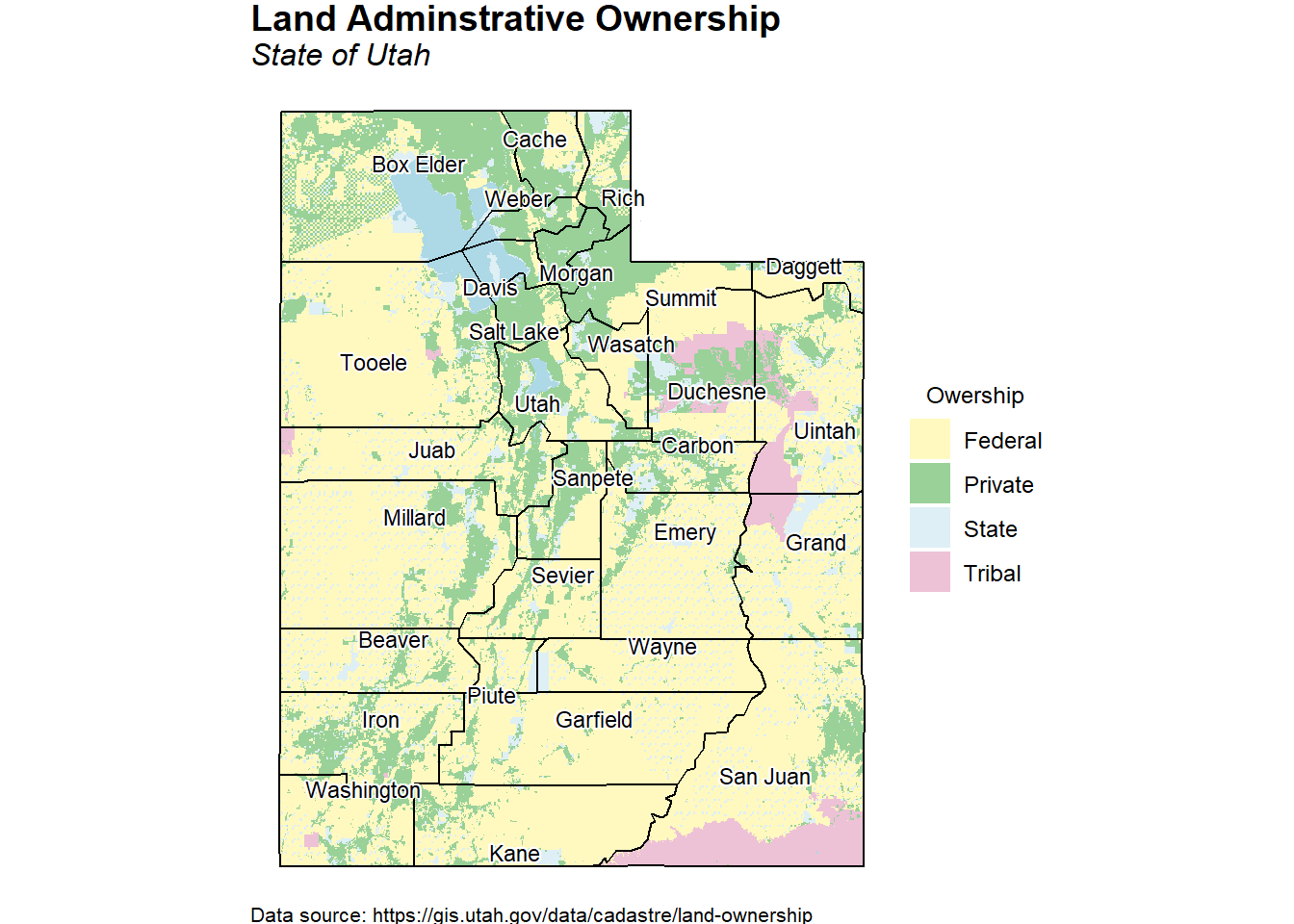
Let’s create a map showing land ownership using the SITLA land ownership data. This statewide dataset is a compilation of all surface land ownership administration and designation categories. Both the SITLA and the Bureau of Land Management (BLM) update this dataset regularly.
# Land ownership map
cols <- c('#FFF062', 'green4', 'lightblue', '#D26799')
ggplot() +
  geom_sf(data = lands, aes(fill = OWNER), color = NA) +
  geom_sf(data = water, color = NA, fill = 'lightblue', size = 0.6, alpha = 1) +
  geom_sf(data = utah_counties, color = 'black', fill = NA) +
  geom_sf_text_repel(data = utah_counties, aes(label = NAME),
                     size = 3, bg.color = 'white', color = 'black') +
  coord_sf(datum = sf::st_crs(utah_counties)) +
  scale_fill_manual(values = alpha(cols, 0.4)) +
  labs(title = 'Land Adminstrative Ownership',
       subtitle = 'State of Utah',
       caption = 'Data source: https://gis.utah.gov/data/cadastre/land-ownership',
       fill = 'Owership') +
  theme_gppr()
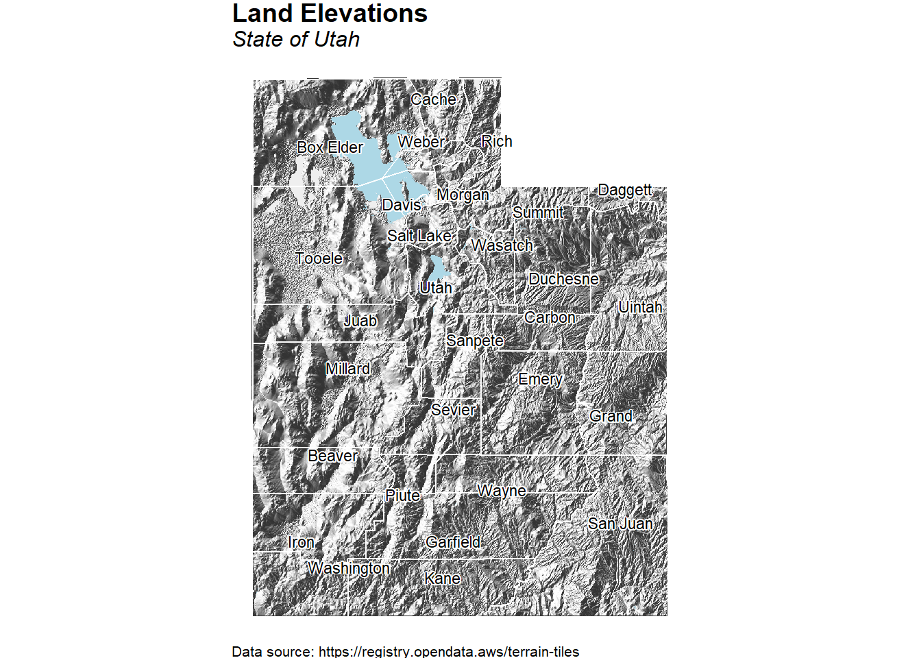
Shaded Relief Map
Let’s create a shaded relief map using the geom_relief() function and the digital elevation data downloaded from the AWS Tiles.
# Elevation map
ggplot() +
  geom_relief(data = elevations,
              aes(x = x, y = y, z = elevation, light = 'white', dark = 'grey20'),
               raster = FALSE, interpolate = TRUE, sun.angle = 60) +
  geom_sf(data = water, color = NA, fill = 'lightblue', size = 0.6, alpha = 1) +
  geom_sf(data = utah_counties, color = 'white', fill = NA) +
  geom_sf_text_repel(data = utah_counties, aes(label = NAME),
                     size = 3, bg.color = 'white', color = 'black') +
  coord_sf(datum = sf::st_crs(utah_counties)) +
  labs(title = 'Land Elevations',
       subtitle = 'State of Utah',
       caption = 'Data source: https://registry.opendata.aws/terrain-tiles',
       fill = 'Owership') +
  theme_gppr()
Land Ownership With Shaded Relief Map - Method 1
Now, let’s create a map showing land ownership using shaded relief as a basemap. Let’s set the geom_relief() light and dark aesthetics to the colors “white” and “grey20”, respectively, and the sun at 60 degrees elevation.
# Create plot
ggplot() +
  geom_relief(data = elevations,
              aes(x = x, y = y, z = elevation, light = 'white', dark = 'grey20'),
               raster = FALSE, interpolate = TRUE, sun.angle = 60) +
  geom_sf(data = lands, aes(fill = OWNER), color = NA) +
  geom_sf(data = water, color = NA, fill = 'lightblue', size = 0.6, alpha = 1) +
  geom_sf(data = utah_counties, color = 'white', fill = NA) +
  geom_sf_text_repel(data = utah_counties, aes(label = NAME),
                     size = 3, bg.color = 'white', color = 'black') +
  coord_sf(datum = sf::st_crs(utah_counties)) +
  scale_fill_manual(values = alpha(cols, 0.3)) +
  labs(title = 'Land Adminstrative Ownership With DEM',
       subtitle = 'State of Utah',
       caption = 'Data source: https://gis.utah.gov/data/cadastre/land-ownership',
       fill = 'Owership') +
  theme_gppr()
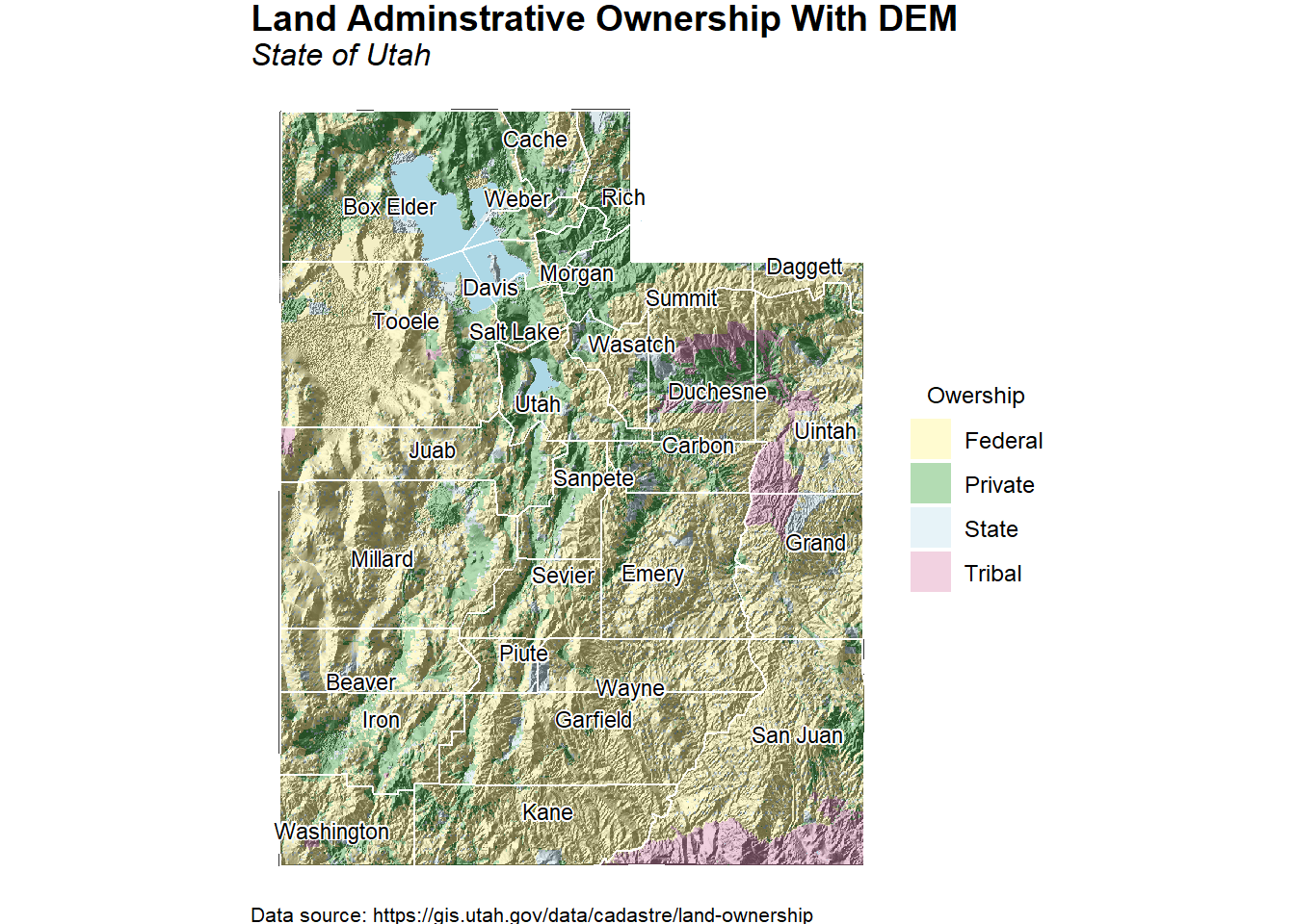
The output looks good, although, some of the minor details of the SITLA land ownership are difficult to discern. This is especially apparent for the small plots of private lands scattered throughout the large area of federal land in Millard county.
Land Ownership With Shaded Relief Map - Method 2
A second method of using shaded relief as a basemap is too assign colors to the light and dark aesthetics based on the land ownership associated for each elevation point. This requires a point-in-polygon analysis using the over() function in the R package sp. First, we need to convert the elevations dataframe with point locations to a SpatialPointsDataFrame and the land ownership shapefile to a sp object. We also need to ensure that the coordinate reference system (CRS) for both the point elevation locations and the lands ownership sp object is the same. Then, we use the over() function to determine which owner polygon contains each elevation point location, and store the owner category id as an attribute of the elevation spatial dataframe. To resolve spherical geometry failures when joining the spatial data, turn off the s2 processing via sf::sf_use_s2(FALSE).
# Increase memory
memory.limit(size = 80000)

# Switch off spherical geometry (s2)
sf_use_s2(FALSE)

# Make elevation data a spatial dataframe
relief <- elevations
coordinates(relief) = ~x+y

# Convert lands from sf to sp object
lands2 <- lands %>%
  dplyr::select(OWNER) %>%
  as(., 'Spatial')

# make sure projections are the same
slot(relief, 'proj4string') <- slot(lands2, 'proj4string')

# Use 'over' with lands2 as a SpatialPolygonsDataFrame object, to determine
# which owner polygon contains each location, and store the owner id as an
# attribute of the relief data
relief$OWNER <- over(relief, lands2)

# Convert relief to dataframe
relief <- as.data.frame(relief)
Now, we can assign colors to the light and dark aesthetics of the geom_relief() function based on the land ownership associated with each elevation point.
relief <- relief %>%
  mutate(
    light = ifelse(OWNER == 'Federal', '#FCFDD4',
              ifelse(OWNER == 'Private', '#B2EFAB',
                ifelse(OWNER == 'State', '#BCF2FA', '#FFE4FC'
                )
              )
            ),
    dark = ifelse(OWNER == 'Federal', '#8F9402',
              ifelse(OWNER == 'Private', '#0E5515',
                ifelse(OWNER == 'State', '#136183', '#66256E'
                )
              )
            )
  )
Finally, let’s create a map showing land ownership using shaded relief as a basemap where colors for the light and dark aesthetics are assigned based on land ownership.
# Create plot
ggplot() +
  geom_sf(data = lands, aes(fill = OWNER), color = NA) +
  geom_relief(data = relief,
              aes(x = x, y = y, z = elevation, light = light, dark = dark),
               raster = FALSE, interpolate = TRUE, sun.angle = 60) +
  geom_sf(data = utah_counties, color = 'white', fill = NA) +
  geom_sf_text_repel(data = utah_counties, aes(label = NAME),
                     size = 3, bg.color = 'white', color = 'black') +
  coord_sf(datum = sf::st_crs(utah_counties)) +
  scale_fill_manual(values = cols) +
  labs(title = 'Land Adminstrative Ownership With DEM',
       subtitle = 'State of Utah',
       caption = 'Data source: https://gis.utah.gov/data/cadastre/land-ownership',
       fill = 'Owership') +
  theme_gppr()
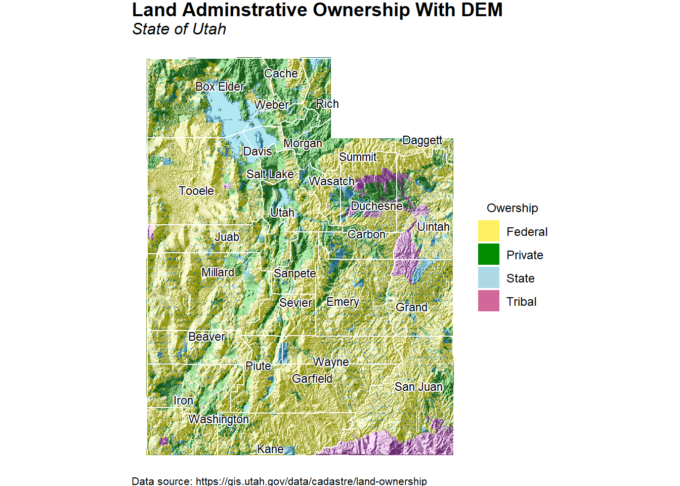
With this new map, the small plots of private lands scattered throughout the large area of federal land in Millard county are now more readily visible.
- Posted on:
- July 25, 2022
- Length:
- 10 minute read, 2084 words
- See Also: