Optimizing Groundwater Monitoring Frequencies Using Temporal Variograms
By Charles Holbert
June 9, 2026
Introduction
Groundwater monitoring programs often seek to optimize sampling frequencies to meet monitoring objectives while minimizing unnecessary sampling costs. Two commonly applied temporal optimization methods are temporal variograms and iterative thinning. Although both approaches evaluate temporal redundancy in monitoring data, they differ substantially in their objectives and implementation.
Iterative thinning directly evaluates information loss by progressively removing sampling events from a monitoring record and assessing whether the remaining data can still reproduce the original concentration trend within predefined confidence limits. Sampling events are removed until the trend can no longer be adequately represented. The interval between the retained sampling events is then used to estimate an optimized sampling frequency.
In contrast, a temporal variogram evaluates how differences in groundwater concentrations change as the time interval between samples increases. The method quantifies temporal correlation within a dataset and identifies a characteristic time range beyond which additional sampling contributes little new information. Because it focuses on temporal dependence rather than trend reconstruction, the variogram approach can be particularly useful when historical monitoring records are relatively limited.
Temporal variograms provide a quantitative framework for estimating sampling frequencies based on the temporal behavior of contaminant concentrations observed in monitoring wells. This post presents an R-based workflow for constructing pooled temporal variograms from nested intrawell concentration pairs and using the resulting variogram model to estimate optimized groundwater sampling intervals.
Background
Temporal variograms identify the sampling lag at which groundwater concentration measurements are no longer temporally correlated. Samples collected at shorter time lags tend to exhibit correlation and therefore contain some degree of statistical redundancy. Unlike a spatial variogram, which assesses similarity as a function of distance, a temporal variogram assesses similarity as a function of time lag. When groundwater concentrations remain relatively stable through time, measurements collected at short intervals are similar and the semivariance remains low. As the lag between samples increases, concentrations typically become less similar, causing semivariance to increase.
For temporal optimization, the variogram should exhibit a recognizable structure characterized by a gradual increase in semivariance with increasing lag, followed by a plateau known as the sill. The lag at which the variogram first reaches the sill is referred to as the range. Beyond the range, concentration measurements are effectively uncorrelated, indicating that samples separated by that amount of time provide largely independent information. Conversely, sampling intervals shorter than the range are associated with correlated, and therefore partially redundant, results.
In this workflow, the variogram range is used as the basis for estimating an optimized sampling interval. A user-defined adjustment factor can then be applied to produce a more conservative sampling frequency where warranted by monitoring objectives or site-specific considerations.
Workflow
The temporal variogram technique is based on the approach presented in the Air Force Civil Engineering Center (AFCEC; formerly AFCEE) Geostatistical Temporal-Spatial (GTS) software (ESTCP, 2010). The method is designed to optimize sampling frequencies simultaneously across a group of monitoring wells for a given constituent of concern (COC). Unlike the original GTS workflow, which often relied on visual interpretation of variogram plots, the R implementation includes an automated sill-detection algorithm. The algorithm evaluates plateau stability using relative slope, relative variability, and relative level criteria and reports when no defensible plateau can be identified within the available range of lag times.
The temporal variogram is constructed using nested pairs of concentration measurements from each well in the group. The pairs are considered nested because they are formed only within individual well locations and never across different wells, which would introduce unwanted spatial variability into the analysis. This approach allows an independent estimate of temporal variability to be obtained from each well.
The nested pairs from all wells are then amalgamated into a single dataset for the entire monitoring network. In this way, wells with more sampling data naturally contribute more pair combinations and therefore receive greater weight in the final temporal variogram, while wells with fewer observations still contribute information but have proportionally less influence. The temporal variogram is a graphical representation of how concentration similarity changes as the time lag between sampling events increases. It provides a quantitative measure of temporal correlation and the rate at which that correlation diminishes through time.
Prior to constructing lag pairs and combining data across wells, concentration measurements are standardized within each well to have a common mean and standard deviation. This standardization improves comparability among wells and helps ensure that temporal patterns are not obscured by differences in concentration magnitude between locations.
To improve the reliability of the estimated temporal pattern, the workflow includes options to exclude older data outside a specified lookback period and to exclude constituent-well combinations with low detection frequencies. In addition, wells with fewer than three distinct sampling events are excluded because they do not provide sufficient information to estimate temporal variability.
The workflow also includes an optional parametric modeling step in which either an exponential or spherical variogram model is fitted to the empirical temporal variogram. The resulting practical range can be used as an alternative estimate of temporal correlation length and compared with the empirical sill-based range estimate. The parametric fit can be useful as a sensitivity check, but it should be interpreted carefully if the empirical curve never stabilizes.
The analysis proceeds through the following steps:
- Prepare the data.
- Standardize concentrations within each well.
- Build nested intrawell pairs.
- Fit the empirical temporal variogram.
- Detect a sill and estimate the temporal range.
- Optionally fit a parametric variogram model.
- Apply a sampling-interval multiplier.
- Return the final sampling frequency recommendation.
The temporal range represents the characteristic time scale over which concentration measurements remain correlated. The script supports three range-selection modes:
auto: use the empirical range when a sill exists, otherwise returnNAnonparametric: always use the empirical rangeparametric: use the practical range from the fitted model
After a raw range is selected, the script applies a user-defined range_multiplier. Practitioners may choose to sample more frequently than the full variogram range to provide earlier detection of concentration changes or to satisfy regulatory and management objectives. For example, applying a multiplier of 0.5 results in a recommended sampling interval equal to one-half of the estimated temporal range. This adjustment does not alter the underlying variogram analysis; rather, it provides a flexible mechanism for translating the estimated temporal correlation structure into a practical monitoring frequency
Example Usage
The following example demonstrates how the temporal variogram workflow can be applied to evaluate sampling frequency for barium across a group of monitoring wells. In this example, the empirical variogram is used as the primary basis for estimating the temporal range, while an exponential variogram model is also fitted for comparison purposes. A sampling-interval multiplier of 0.5 is applied, meaning the recommended sampling interval is one-half of the estimated temporal range. This provides a more conservative monitoring frequency than using the full variogram range and may be appropriate when earlier detection of concentration changes is desired.
The analysis is performed using the following code:
# Load functions
source("functions/temporal_variogram_optimize_v2.R")

# Load data
exdata <- readr::read_csv("data/exdata.csv", show_col_types = FALSE)

# Run temporal optimization for barium
res <- temporal_variogram_group(
  input_df = exdata,
  coc = "Barium",
  range_method = "auto", # "parametric", "nonparametric", or "auto"
  parametric_model = "exponential",
  range_multiplier = 0.5
)

# Inspect results
res$parametric_converged
## [1] TRUE
res$no_sill
## [1] FALSE
res$no_sill_reason
## [1] NA
res$raw_selected_range_days
## [1] 1065.8
res$range_multiplier
## [1] 0.5
res$selected_range_days
## [1] 532.9
res$selected_range_quarters
## [1] 6
print(res$plot)
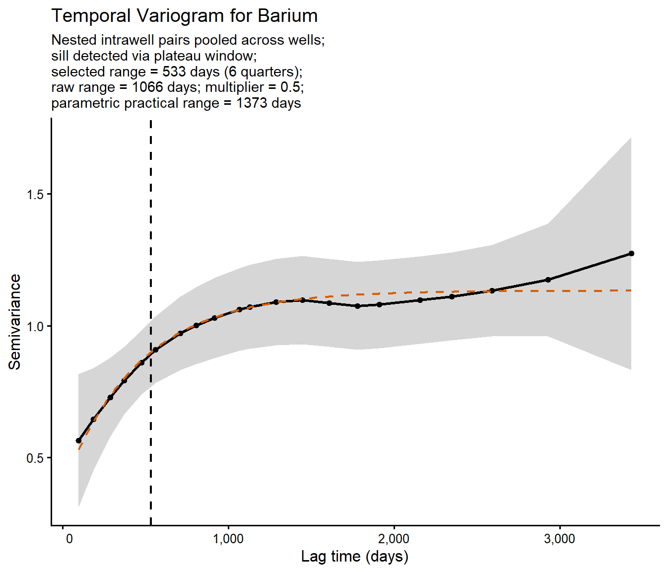
The empirical variogram exhibits a clear sill, indicating that temporal correlation decreases and eventually stabilizes as the lag between sampling events increases. The plateau-detection algorithm identified a temporal range of approximately 1,066 days, while the fitted exponential model produced a practical range of approximately 1,373 days. Applying the 0.5 multiplier resulted in a recommended sampling interval of approximately 533 days (about 6 calendar quarters). The close agreement between the empirical and parametric estimates provides additional confidence that the observed temporal structure is reasonably well defined and that the recommended sampling interval is supported by the available monitoring data.
The barium example demonstrates a case in which the temporal variogram exhibits a clear sill and a corresponding temporal range could be identified. The following example illustrates the opposite situation using cobalt, where the available monitoring data do not provide sufficient evidence of a stable temporal plateau.
The analysis is performed using the same workflow and settings:
# Run temporal optimization for cobalt
res <- temporal_variogram_group(
  input_df = exdata,
  coc = "Cobalt",
  range_method = "auto", # "parametric", "nonparametric", or "auto"
  parametric_model = "exponential",
  range_multiplier = 0.5
)

# Inspect results
res$parametric_converged
## [1] TRUE
res$no_sill
## [1] TRUE
res$no_sill_reason
## [1] "no_plateau_window"
res$raw_selected_range_days
## [1] NA
res$range_multiplier
## [1] 0.5
res$selected_range_days
## [1] NA
res$selected_range_quarters
## [1] NA
print(res$plot)
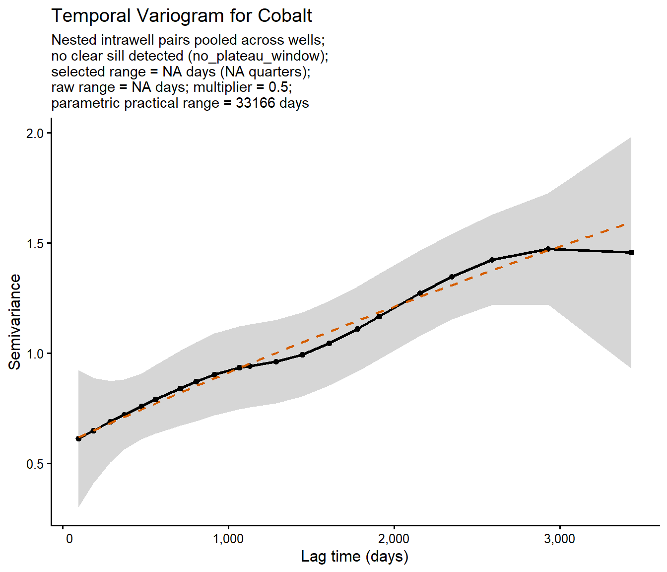
In this example, the empirical temporal variogram continues to increase with increasing lag time and does not exhibit a sufficiently stable plateau region. Although the variogram begins to flatten at longer lag times, the plateau-detection algorithm was unable to identify a sill that satisfied the stability criteria used by the workflow. As a result, no empirical temporal range was identified.
The fitted exponential variogram model did converge and produced a practical range estimate of approximately 33,166 days. However, this estimate should be interpreted cautiously because the empirical variogram does not exhibit a well-defined sill within the range of observed lag times. In this situation, the fitted model is effectively extrapolating beyond the available data, resulting in a practical range estimate that is much larger than the observed temporal extent of the monitoring record.
This example highlights an important strength of the workflow. Rather than forcing a sampling recommendation when temporal structure is poorly defined, the empirical variogram analysis explicitly reports that no defensible temporal range could be identified. This outcome indicates that the available data do not provide sufficient evidence of a characteristic temporal correlation length and that a temporal-variogram-based sampling frequency cannot be determined with confidence using the current dataset.
Conclusions
Temporal variograms offer a practical, statistically grounded approach for evaluating groundwater sampling frequency. By using nested intrawell pairs, standardizing concentrations within wells, and estimating a temporal range from pooled monitoring data, the workflow provides a quantitative basis for sampling frequency decisions. When a sill is present, the estimated range can be used directly or scaled using a sampling-interval multiplier to produce a more conservative monitoring frequency. When a sill cannot be identified, the workflow appropriately avoids forcing a recommendation that is not supported by the available data.
In practice, temporal variograms do not always clearly identify a range (i.e., the smallest sampling lag associated with negligible temporal correlation). Successful application of the method generally requires that:
- Sample pairs exist in sufficient quantity across a broad range of lag times so that potential sampling intervals are adequately represented.
- Concentration levels at most wells are reasonably stable over time, but not completely constant, so that temporal correlations can be estimated without being dominated by long-term trends.
- The dataset is not dominated by non-detects or wells with little to no concentration variability. When concentration histories are largely constant, there is insufficient information to relate concentration behavior to sampling lag.
When these conditions are not met, temporal variograms may fail to identify a defensible sill and range, limiting their usefulness for sampling optimization.
Comparative evaluations have shown that iterative thinning often provides more reliable and reproducible sampling frequency recommendations than temporal variograms. Temporal variograms are best viewed as a screening or exploratory tool that helps characterize temporal correlation within a monitoring network. Iterative thinning, by contrast, directly evaluates the information loss associated with reducing sampling frequency and quantifies the impact of sampling reduction on the ability to reproduce historical concentration trends. For this reason, iterative thinning is frequently preferred when developing final sampling frequency recommendations, while temporal variograms can provide valuable supporting evidence regarding the temporal behavior of groundwater concentrations.
The following table summarizes the primary differences between temporal variograms and iterative thinning, including their underlying objectives, data requirements, scale of application, and typical use in groundwater monitoring optimization.
| Aspect | Temporal Variogram | Iterative Thinning |
|---|---|---|
| Scale | Group of wells | Individual well |
| Output | One sampling interval for the entire group | Optimal interval for each well |
| Core idea | Measure how quickly samples lose temporal correlation | Test how much data can be removed while preserving the trend |
| Data requirement | Works with shorter histories | Requires more data (typically ≥8 samples/well) |
| Handles seasonal/nonlinear trends well? | Not very well | Yes |
| User involvement | User identifies the variogram range | Mostly automated |
| Performance in testing | Mixed to poor | Strong and reproducible |
References
Environmental Security Technology Certification Program (ESTCP). 2010. Demonstration and Validation of the Geostatistical Temporal-Spatial Algorithm (GTS) for Optimization of Long-Term Monitoring (LTM) of Groundwater at Military and Government Sites. U.S. Department of Defense ESTCP Cost and Performance Report ER-200714. August.
Appendix: Core Functions
The analysis is organized around the following functions:
##  [1] "build_nested_pairs"              "build_nested_pairs_v3"
##  [3] "build_variogram_bins"            "estimate_nonparametric_range"
##  [5] "estimate_nonparametric_range_v3" "fit_parametric_practical_range"
##  [7] "fit_temporal_variogram"          "fit_temporal_variogram_v3"
##  [9] "make_parametric_curve"           "parse_any_date"
## [11] "prepare_temporal_variogram_data" "prepare_tv_data_v3"
## [13] "quarter_from_days"               "safe_sd01"
## [15] "temporal_variogram_group"        "temporal_variogram_group_v3"
- Posted on:
- June 9, 2026
- Length:
- 11 minute read, 2154 words
- See Also: