Derivation of a Power Expression for Trend Detection Under AR(1) Noise
By Charles Holbert
May 12, 2026
Introduction
Detecting long-term environmental trends is fundamentally a signal-to-noise problem. In many environmental, hydrological, and climatological applications, the underlying trend is often small relative to the magnitude of natural variability, and the observational record may contain substantial temporal autocorrelation. As a consequence, even physically meaningful trends may remain statistically undetectable unless the monitoring record is sufficiently long.
A rigorous framework for evaluating trend detectability was developed in the influential work of Weatherhead et al. (1998), which demonstrated that the number of observations required to detect a trend depends primarily on four quantities: the trend magnitude, the variance of the residual noise, the degree of autocorrelation, and the desired statistical confidence level. The Weatherhead-style approach, building on earlier work examining the effects of autocorrelation and temporal sampling on environmental trend estimation (Tiao et al. 1990), has since become widely used in atmospheric science, climatology, hydrology, and environmental monitoring because it provides a practical means of estimating the observational record length necessary to achieve reliable trend detection.
The key insight of the Weatherhead framework is that autocorrelation substantially reduces the effective amount of independent information contained in a time series. Positive serial correlation inflates the variance of estimated trends and therefore increases the number of years required to detect statistically significant change. Consequently, trend detectability cannot be evaluated solely on the basis of trend magnitude and variance; the temporal structure of the residual process must also be considered explicitly.
The present work develops an approximate analytical framework for evaluating statistical power and sample-size requirements for Mann-Kendall type trend analyses under AR(1) residual structure. Using large-sample asymptotic approximations, analytical expressions are derived for trend-estimator variance, statistical power, and required sample size as functions of trend magnitude, residual variability, serial autocorrelation, statistical significance level, and record length. Unlike traditional Weatherhead-style formulations focused primarily on regression-based detection times, the present framework develops explicit analytical power and sample-size relationships within a Mann-Kendall oriented trend-detection context while retaining the influence of AR(1) residual autocorrelation.
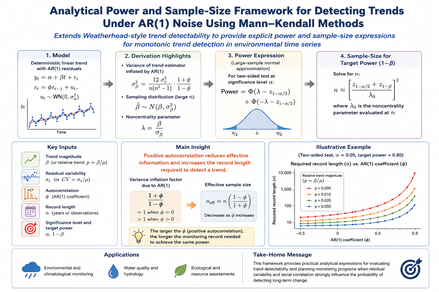
The figure below provides a graphical overview of the analytical framework developed in this study, illustrating the relationships among trend magnitude, residual variability, serial autocorrelation, statistical power, and required monitoring duration for Mann-Kendall type trend detection under AR(1) residual behavior.
Background and Statistical Framework
The present derivation follows this general Weatherhead-style trend-detectability framework while focusing specifically on approximate power expressions relevant to Mann-Kendall-type monotonic trend analyses. The derivation assumes that the observed time series consists of a deterministic linear trend superimposed on a first-order autoregressive [AR(1)] residual process. Using large-sample normal approximations, analytical expressions are derived for:
- variance of the trend estimator under AR(1) residual noise,
- statistical power of detecting a monotonic trend,
- influence of autocorrelation on trend detectability, and
- sample size required to achieve a specified statistical power.
Mann-Kendall Trend Detection
Although the Mann-Kendall test is formally nonparametric, its large-sample behavior is asymptotically related to regression-based trend estimation and associated monotonic slope estimators such as the Theil-Sen estimator (Theil 1950; Sen 1968). Under large-sample conditions, the standardized Mann-Kendall statistic converges asymptotically to a normal distribution. Consequently, approximate power expressions may be derived using the same noncentrality concepts commonly applied to regression-based trend estimators. The resulting approximations therefore provide a practical analytical framework for evaluating trend detectability in environmental monitoring applications where residual variability and autocorrelation strongly influence the probability of detecting long-term change. In this context, trend detectability is quantified through statistical power, defined as the probability of correctly rejecting the null hypothesis of no trend when a true trend exists.
AR(1) Residual Framework
The resulting equations provide a compact and practical framework for estimating the number of observations required to detect trends of specified magnitude in environmental time series exhibiting approximately AR(1) residual behavior. Although higher-order and nonstationary residual processes may occur in practice, the AR(1) assumption provides a tractable first-order approximation widely used in environmental trend-detection studies.
The derivation follows the large-sample approximations commonly used in trend-detection and Weatherhead-style trend-detectability studies, and yields an approximate analytical power expression applicable to Mann-Kendall-type monotonic trend analyses (Mann 1945; Kendall 1975) through the asymptotic equivalence between monotonic trend tests and regression-based slope estimation. Under large-sample conditions, the standardized Mann-Kendall statistic converges asymptotically to a normal distribution, allowing approximate power relationships to be derived using noncentrality concepts analogous to those used in regression-based trend estimation.
Trend Model with AR(1) Residuals
Consider a time series consisting of a deterministic linear trend and a stochastic residual component. The objective is to derive an approximate analytical expression for the statistical power of detecting a monotonic trend in the presence of first-order autocorrelated noise and to obtain the corresponding sample-size requirement for a specified power level.
The observed time series is modeled as:
\begin{equation}\tag{1} y_t = \beta t + \varepsilon_t \end{equation}
where
\(y_t\)denotes the observed value at time index\(t\),\(t = 1,\ldots,n\),\(n\)is the sample size,\(\beta\)is the true linear trend slope, and\(\varepsilon_t\)is the stochastic residual term.
The residual process is assumed to follow a stationary first-order autoregressive [AR(1)] process,
\begin{equation}\tag{2} \varepsilon_t = \phi \varepsilon_{t-1} + a_t, \qquad |\phi| < 1 \end{equation}
where
\(\phi\)is the lag-1 autocorrelation coefficient,\(a_t\)are independent Gaussian innovations,\(a_t \sim N(0,\sigma_a^2)\), and\(\sigma_a^2\)is the innovation variance.
The stationarity condition is
\begin{equation}\tag{3} -1 < \phi < 1 \end{equation}
When \(\phi=0\), the residuals are serially independent. Positive values (\(0<\phi<1\)) indicate positive serial correlation, producing persistence in the time series, whereas negative values (\(-1<\phi<0\)) indicate alternating behavior between successive observations. As \(|\phi|\) approaches 1, the process becomes increasingly persistent and approaches nonstationarity. Typical values encountered in environmental and climatological applications are approximately:
| Degree of autocorrelation | Approximate `\(\phi\)` |
|---|---|
| Independent residuals | 0.0 |
| Weak autocorrelation | 0.1--0.3 |
| Moderate autocorrelation | 0.3--0.6 |
| Strong autocorrelation | 0.6--0.9 |
The autocorrelation factor that enters the power expression is
\begin{equation}\tag{4} \sqrt{\frac{1-\phi}{1+\phi}} \end{equation}
This factor decreases as \(\phi\) increases. Consequently, positive autocorrelation reduces statistical power because it lowers the effective amount of independent information in the time series. This reduction in effective information content due to serial correlation is closely related to effective-sample-size approaches developed for modified Mann-Kendall testing (Yue and Wang 2004). Representative values are shown below.
| `\(\phi\)` | `\(\sqrt{(1-\phi)/(1+\phi)}\)` |
|---|---|
| 0.0 | 1.000 |
| 0.3 | 0.734 |
| 0.5 | 0.577 |
| 0.7 | 0.420 |
| 0.9 | 0.229 |
Variance of AR(1) Residual Process
The variance structure of the AR(1) residual process determines how serial correlation influences the uncertainty of estimated trends. The following derivation relates the innovation variance to the stationary variance of the residual process and provides the autocorrelation scaling factor that later enters the power expression.
Under stationarity,
\begin{equation}\tag{5} Var(\varepsilon_t) = Var(\varepsilon_{t-1}) = \sigma_\varepsilon^2 \end{equation}
where \(\sigma_\varepsilon^2\) denotes the variance of the residual process.
Taking the variance of both sides of equation (2) yields
\begin{equation}\tag{6} Var(\varepsilon_t) = \phi^2 Var(\varepsilon_{t-1}) + Var(a_t) \end{equation}
Substituting equation (3) into equation (6) gives
\begin{equation}\tag{7} \sigma_\varepsilon^2 = \phi^2 \sigma_\varepsilon^2 + \sigma_a^2 \end{equation}
Solving equation (7) for \(\sigma_\varepsilon^2\) produces
\begin{equation}\tag{8} \sigma_\varepsilon^2 = \frac{\sigma_a^2}{1-\phi^2} \end{equation}
Equivalently,
\begin{equation}\tag{9} \sigma_a^2 = \sigma_\varepsilon^2(1-\phi^2) \end{equation}
Equation (8) shows that positive serial correlation inflates the variance of the residual process relative to the innovation variance. The influence of serial correlation on Mann-Kendall-type trend detection has been extensively discussed in the hydrological literature (Hamed and Rao 1998).
Standard Error of Estimated Trend
Let \(\hat{\beta}\) denote the estimated linear trend slope. For large sample sizes, the standard deviation of the estimated slope under AR(1) residual noise may be approximated as
\begin{equation}\tag{10} \sigma_{\hat{\beta}} \approx \frac{\sigma_\varepsilon}{n^{3/2}} \sqrt{\frac{1+\phi}{1-\phi}} \end{equation}
where \(\sigma_{\hat{\beta}}\) denotes the standard deviation of the slope estimator. Equation (10) represents a large-sample approximation commonly used in trend-detectability analyses for approximately equally spaced observations with stationary AR(1) residual structure. The approximation is consistent with the Weatherhead-style framework commonly applied in environmental and climatological trend-detection studies. Equation (10) indicates that positive autocorrelation (\(\phi>0\)) increases the uncertainty associated with the estimated trend slope by inflating the variance of the estimator and reducing the effective amount of independent information contained in the time series.
Distribution of Trend Estimator
To derive analytical power expressions, the sampling distribution of the estimated trend slope must be specified. Under large-sample conditions, the slope estimator is assumed to be approximately normally distributed with mean equal to the true trend and variance determined by the AR(1) residual structure.
Assuming asymptotic normality of the slope estimator,
\begin{equation}\tag{11} \hat{\beta} \sim N(\beta,\sigma_{\hat{\beta}}^2) \end{equation}
where \(\beta\) is the true slope.
Define the standardized test statistic
\begin{equation}\tag{12} T = \frac{\hat{\beta}}{\sigma_{\hat{\beta}}} \end{equation}
Using equation (11), the distribution of \(T\) is
\begin{equation}\tag{13} T \sim N\left( \frac{\beta}{\sigma_{\hat{\beta}}} 1 \right) \end{equation}
Define the noncentrality parameter
\begin{equation}\tag{14} \delta = \frac{\beta}{\sigma_{\hat{\beta}}} \end{equation}
Substituting equation (10) into equation (14) yields
\begin{equation}\tag{15} \delta = \frac{\beta n^{3/2}}{\sigma_\varepsilon} \sqrt{\frac{1-\phi}{1+\phi}} \end{equation}
The \(n^{3/2}\) dependence arises because the variance of the estimated linear trend decreases approximately as \(n^{-3}\) under large-sample linear-trend estimation. Equation (15) demonstrates that detectability increases with increasing trend magnitude and sample size, and decreases with increasing residual variability and autocorrelation.
Power of One-Sided Trend Test
Consider the one-sided hypothesis test
\begin{equation}\tag{16} H_0:\beta=0, \qquad H_1:\beta>0 \end{equation}
At significance level \(\alpha\), the null hypothesis is rejected when
\begin{equation}\tag{17} T>z_{1-\alpha} \end{equation}
where \(z_{1-\alpha}\) denotes the \((1-\alpha)\)-quantile of the standard normal distribution.
The statistical power is therefore
\begin{equation}\tag{18} \text{Power} = P(T>z_{1-\alpha}\mid \beta) \end{equation}
Using equation (13), equation (18) becomes
\begin{equation}\tag{19} \text{Power} = \Phi(\delta-z_{1-\alpha}) \end{equation}
where \(\Phi(\cdot)\) denotes the cumulative distribution function of the standard normal distribution.
Substituting equation (15) into equation (19) gives
\begin{equation}\tag{20} \text{Power} = \Phi \left[ \frac{\beta n^{3/2}}{\sigma_\varepsilon} \sqrt{\frac{1-\phi}{1+\phi}} - z_{1-\alpha} \right] \end{equation}
Equation (20) provides the approximate statistical power for detecting a positive monotonic trend in the presence of AR(1) residual noise.
Power of Two-Sided Trend Test
For a two-sided test,
\begin{equation}\tag{21} H_0:\beta=0, \qquad H_1:\beta\neq0 \end{equation}
the rejection region becomes
\begin{equation}\tag{22} |T|>z_{1-\alpha/2} \end{equation}
where \(z_{1-\alpha/2}\) denotes the \((1-\alpha/2)\)-quantile of the standard normal distribution.
The corresponding power is given by:
\begin{equation}\tag{23} \text{Power} = P(|T|>z_{1-\alpha/2}\mid \beta) \end{equation}
Using equation (13),
\begin{equation}\tag{24} \text{Power} = 1 - \Phi(z_{1-\alpha/2}-\delta) + \Phi(-z_{1-\alpha/2}-\delta) \end{equation}
For positive trends and moderate-to-large values of \(\delta\), the final term in equation (24) is typically negligible.
Power in Terms of Relative Trend Magnitude
For many environmental applications, it is more useful to express trend magnitude and residual variability relative to the mean level of the observed series. The following formulation rewrites the power expression in terms of fractional trend magnitude and the coefficient of variation, producing a dimensionless representation of trend detectability.
Let
\begin{equation}\tag{25} \mu = \text{mean level of the series} \end{equation}
and define the fractional trend rate as
\begin{equation}\tag{26} p=\frac{\beta}{\mu} \end{equation}
where \(p\) represents the fractional change per unit time.
Define the coefficient of variation of the residual variability as
\begin{equation}\tag{27} CV=\frac{\sigma_\varepsilon}{\mu} \end{equation}
Using equations (26) and (27),
\begin{equation}\tag{28} \frac{\beta}{\sigma_\varepsilon} = \frac{p}{CV} \end{equation}
Substituting equation (28) into equation (20) yields
\begin{equation}\tag{29} \text{Power} = \Phi \left[ \frac{p}{CV} n^{3/2} \sqrt{\frac{1-\phi}{1+\phi}} - z_{1-\alpha} \right] \end{equation}
Equation (29) expresses statistical power in terms of relative trend magnitude and relative residual variability.
Sample Size Required for Specified Power
Let the desired statistical power be \(1-\beta_{\mathrm{II}}\), where \(\beta_{\mathrm{II}}\) denotes the Type II error probability. Equation (29) may then be written as
\begin{equation}\tag{30} 1-\beta_{\mathrm{II}} = \Phi \left[ \frac{p}{CV} n^{3/2} \sqrt{\frac{1-\phi}{1+\phi}} - z_{1-\alpha} \right] \end{equation}
Applying the inverse standard normal cumulative distribution function to equation (30) gives
\begin{equation}\tag{31} z_{1-\beta_{\mathrm{II}}} = \frac{p}{CV} n^{3/2} \sqrt{\frac{1-\phi}{1+\phi}} - z_{1-\alpha} \end{equation}
Solving equation (31) for \(n\) yields
\begin{equation}\tag{32} n = \left[ \frac{z_{1-\alpha}+z_{1-\beta_{\mathrm{II}}}}{p/CV} \sqrt{\frac{1+\phi}{1-\phi}} \right]^{2/3} \end{equation}
or equivalently,
\begin{equation}\tag{33} n = \left[ \frac{(z_{1-\alpha}+z_{1-\beta_{\mathrm{II}}}) CV}{p} \sqrt{\frac{1+\phi}{1-\phi}} \right]^{2/3} \end{equation}
For analyses intended to detect either positive or negative trends, \(p\) may be replaced by \(|p|\).
Equation (33) demonstrates that the required sample size increases with increasing residual variability and increasing serial correlation, and decreases with increasing trend magnitude.
Conclusions
This derivation demonstrates that statistical power for detecting monotonic trends in autocorrelated environmental time series depends primarily on four quantities: trend magnitude, residual variability, serial autocorrelation, and record length. Positive autocorrelation reduces the effective information content of a time series by inflating the variance of the estimated trend slope. Consequently, stronger serial correlation requires larger sample sizes to achieve equivalent statistical power for trend detection.
The resulting expressions provide a practical analytical approximation for evaluating trend detectability in environmental and climatological time series exhibiting approximately AR(1) residual behavior. Unlike traditional Weatherhead-style formulations focused primarily on regression-based detection times, the present framework develops explicit analytical power and sample-size relationships within a Mann-Kendall oriented trend detection context while retaining the influence of AR(1) residual autocorrelation. The framework remains consistent with the Weatherhead-style trend-detectability approach widely used in atmospheric and environmental sciences, while extending that framework through explicit large-sample power formulations applicable to Mann-Kendall-type monotonic trend analyses.
The derivation is based on large-sample asymptotic approximations and assumes approximately linear trends with stationary AR(1) residual behavior. Accordingly, the resulting expressions should be interpreted as practical analytical approximations rather than exact finite-sample results, and are expected to be most reliable for moderate-to-large sample sizes typical of long-term environmental monitoring records. For small samples, actual statistical power may differ from the analytical approximation, autocorrelation effects may be under- or overestimated, and Type I error control may deviate from nominal levels. In such settings, simulation-based approaches may provide more accurate estimates of statistical power and required monitoring duration.
Nevertheless, the analytical framework remains highly useful because environmental trend-detection studies frequently involve long observational records for which large-sample approximations are appropriate. The resulting expressions provide physical and statistical insight into the relationships among trend magnitude, residual variability, serial autocorrelation, statistical power, and monitoring duration, while also enabling rapid sensitivity analyses without requiring computationally intensive Monte-Carlo simulations. These practical advantages are among the reasons Weatherhead-style trend-detectability methods have become widely used in environmental and climatological applications.
Future extensions could consider seasonal structure, nonstationary residual processes, missing observations, irregular sampling intervals, and higher-order autocorrelation models.
References
Hamed, K.H. and Rao, A.R. 1998. A modified Mann-Kendall trend test for autocorrelated data. Journal of Hydrology 204, 182-196.
Kendall, M.G. 1975. Rank Correlation Techniques, 4th ed. Charles Griffen. London.
Mann, H.B. 1945. Nonparametric tests against trend. Econometrica 13, 245-259.
Sen, P.K. 1968. Estimates of the regression coefficient based on Kendall’s Tau. JASA 63, 1379-1389.
Theil, H. 1950. A rank-invariant method of linear and polynomial regression analysis. I-III.Proc. Kon. Ned. Akad. v. Wetensch. A.53 386-392, 521-525, 1397-1412.
Tiao, G.C., Reinsel, G.C., Xu, D., Pedrick, J.H., Zhu, X., Miller, A.J., DeLuisi, J.J., Mateer, C.L., and Wuebbles, D.J. 1990. Effects of autocorrelation and temporal sampling schemes on estimates of trend and spatial correlation. Journal of Geophysical Research 95, 20507-20517.
Weatherhead, E.C., Reinsel, G.C., Tiao, G.C., Meng, X.L., Choi, D., Cheang, W.K., Keller, T., DeLuisi, J., Wuebbles, D.J., Kerr, J.B., Miller, A.J., Oltmans, S.J., and Frederick, J.E. 1998. Factors affecting the detection of trends: Statistical considerations and applications to environmental data. Journal of Geophysical Research: Atmospheres 103, 17149-17161.
Yue, S. and Wang, C.Y. 2004. The Mann-Kendall test modified by effective sample size to detect trend in serially correlated hydrological series. Water Resources Management 18 201-218.
- Posted on:
- May 12, 2026
- Length:
- 12 minute read, 2444 words
- See Also: