Temporal Behavior of Arctic Sea Ice
By Charles Holbert
February 22, 2024
Introduction
The decline of Arctic sea ice due to anthropogenic warming is a critical issue with far-reaching implications for the environment, ecosystems, and human society. Sea ice is frozen seawater that forms in cold, high latitude regions where there is little sunlight in the winter. It plays a crucial role in regulating heat and momentum transfer between the atmosphere and the ocean, as well as acting as a barrier for freshwater, gases, and aerosols. Minor changes in the atmosphere and ocean can significantly impact the annual cycle of sea ice melting and freezing, indicating that sea ice fluctuations reflect the combined changes occurring in both the ocean and atmosphere.
Arctic sea ice serves as a sensitive indicator of climate change. The rapid decline in Arctic sea ice has profound consequences for marine ecosystems, wildlife survival, and indigenous communities (Huntington et al. 2017; Laidre et al. 2020), while also contributing to rising sea levels and extreme weather events globally (Screen and Simmonds 2010). Reduction in the reflective ice surface amplifies the absorption of solar energy by the ocean, which further accelerates global warming (Pistone et al. 2019). Changes to the seasonal cycle of Arctic sea ice can also affect the salinity and density of the surrounding ocean which can have wider impacts for large-scale ocean circulation (Timmermans and Marshall 2020).
Researchers (Vinnikov et al. 1999; Gregory et al. 2002; Min et al. 2008) have found that observed trends in Arctic sea ice are influenced by anthropogenic forces, rather than being solely due to internal variability. Models that include human influences align with observations, in contrast to those relying on natural factors. The correlation between Arctic sea ice trends and atmospheric CO2 supports the impact of human activities (Notz and Marotzke 2012). As the Arctic warms at 3 to 4 times faster than the global average (Rantanen et al. 2022), addressing these changes becomes increasingly important, emphasizing the interconnectedness of the polar climate system and the need for continued research and action to mitigate further impacts (Cohen et al. 2014).
In this blog post, temporal changes in the Arctic sea ice extent (ASIE) will be explored using the R language for statistical computing and visualization.
Preliminaries
Several R libraries will be used for data processing, visualization, and statistical analyses. Those are loaded below. Additionally, two lists are created: an ordered list of names for the months of the year and a list containing common theme elements that will be used when plotting the data.
# Load libraries
library(dplyr)
library(readr)
library(tidyr)
library(lubridate)
library(ggplot2)
library(scales)
library(viridis)
library(fasstr)
library(ggseas)
library(forecast)

# Create list of months
mon <- c(
  'Jan', 'Feb', 'Mar', 'Apr', 'May', 'Jun',
  'Jul', 'Aug', 'Sep', 'Oct', 'Nov', 'Dec'
)

# List of common theme elements for plotting
my_theme <- list(
  theme(plot.title = element_text(margin = margin(b = 3), size = 14,
                       hjust = 0, color = 'black', face = 'bold'),
        plot.subtitle = element_text(margin = margin(b = 4), size = 12,
                          hjust = 0, color = 'black', face = 'italic'),
        plot.caption = element_text(size = 9),
        axis.title = element_text(size = 12, color = 'black'),
        axis.text = element_text(size = 10, color = 'black'),
        legend.justification = c(0, 0),
        legend.position = c(0.03, 0.05),
        plot.margin = unit(c(0.15, 0.25, 0.15, 0.15), 'in'))
)
Data
Scientists use sea ice extent to quantify the amount of sea ice at the poles, which is the total area of ocean with at least 15% ice concentration. Data on sea ice extent is available from the National Snow and Ice Data Center (NSIDC) at the University of Colorado. The NSIDC researches the impact of Earth’s frozen parts on the planet and society, with a focus on the cryosphere elements like snow, ice, glaciers, and frozen ground. The NSIDC sea ice extent data are derived from measurements taken by the passive microwave sensors onboard the Defense Meteorological Satellite Program (DMSP) F8, F11, and F13, and F17 satellites. The data are generated by the NASA Goddard Space Flight Center, with uncertainties in the range of 0.03-0.05 million square kilometers (Meier et al. 2014).
Numeric data used in this post are ASIE, in millions of square kilometers, for the Northern hemisphere from 26 October 1978 through 14 February 2024. The data were previously downloaded from the National Snow and Ice Data Center (NSIDC) and saved as a comma-delimited file. A summary of these data are provided below.
# Load data
dat <- read_csv('data/SeaIce_Daily_Extent_G02135_v3.0.csv')

# Summary of data using skimr
skimr::skim(dat)
Table: Table 1: Data summary
| Name | dat |
| Number of rows | 366 |
| Number of columns | 49 |
| _______________________ | |
| Column type frequency: | |
| numeric | 49 |
| ________________________ | |
| Group variables | None |
Variable type: numeric
| skim_variable | n_missing | complete_rate | mean | sd | p0 | p25 | p50 | p75 | p100 | hist |
|---|---|---|---|---|---|---|---|---|---|---|
| month | 0 | 1.00 | 6.51 | 3.46 | 1.00 | 4.00 | 7.00 | 9.75 | 12.00 | ▇▅▅▅▇ |
| day | 0 | 1.00 | 15.76 | 8.82 | 1.00 | 8.00 | 16.00 | 23.00 | 31.00 | ▇▇▇▇▆ |
| 1978 | 332 | 0.09 | 12.49 | 1.33 | 10.23 | 11.35 | 12.66 | 13.64 | 14.59 | ▇▆▇▅▇ |
| 1979 | 184 | 0.50 | 12.32 | 3.19 | 6.89 | 9.63 | 12.81 | 15.49 | 16.64 | ▅▃▃▅▇ |
| 1980 | 183 | 0.50 | 12.33 | 2.97 | 7.53 | 9.59 | 12.71 | 15.17 | 16.30 | ▆▃▃▅▇ |
| 1981 | 183 | 0.50 | 12.14 | 2.98 | 6.90 | 9.33 | 12.82 | 14.97 | 15.80 | ▅▂▃▃▇ |
| 1982 | 184 | 0.50 | 12.44 | 3.00 | 7.16 | 9.89 | 12.87 | 15.26 | 16.32 | ▅▃▃▅▇ |
| 1983 | 183 | 0.50 | 12.34 | 2.91 | 7.20 | 9.89 | 12.77 | 14.96 | 16.41 | ▅▃▅▆▇ |
| 1984 | 183 | 0.50 | 11.91 | 2.99 | 6.40 | 9.28 | 12.53 | 14.69 | 15.81 | ▅▃▃▅▇ |
| 1985 | 184 | 0.50 | 11.99 | 3.19 | 6.49 | 9.00 | 12.65 | 15.10 | 16.16 | ▅▂▃▃▇ |
| 1986 | 183 | 0.50 | 12.21 | 2.88 | 7.12 | 9.83 | 12.59 | 14.99 | 16.16 | ▅▃▅▅▇ |
| 1987 | 146 | 0.60 | 11.40 | 3.16 | 6.89 | 8.57 | 11.27 | 14.64 | 16.29 | ▇▅▅▃▇ |
| 1988 | 12 | 0.97 | 12.09 | 2.98 | 7.05 | 9.38 | 12.45 | 15.05 | 16.31 | ▆▃▅▅▇ |
| 1989 | 1 | 1.00 | 11.97 | 2.89 | 6.89 | 9.52 | 12.69 | 14.66 | 15.77 | ▅▃▃▆▇ |
| 1990 | 1 | 1.00 | 11.69 | 3.29 | 6.01 | 8.98 | 12.28 | 14.67 | 16.25 | ▆▃▅▅▇ |
| 1991 | 1 | 1.00 | 11.75 | 3.06 | 6.26 | 9.19 | 12.49 | 14.61 | 15.65 | ▅▂▃▅▇ |
| 1992 | 0 | 1.00 | 12.11 | 2.76 | 7.16 | 9.75 | 12.69 | 14.63 | 15.58 | ▅▃▃▅▇ |
| 1993 | 1 | 1.00 | 11.92 | 3.20 | 6.16 | 9.05 | 12.38 | 15.08 | 16.05 | ▅▃▃▅▇ |
| 1994 | 1 | 1.00 | 12.01 | 2.96 | 6.93 | 9.35 | 12.57 | 14.78 | 15.77 | ▅▂▃▃▇ |
| 1995 | 1 | 1.00 | 11.42 | 3.25 | 6.01 | 8.51 | 12.10 | 14.48 | 15.38 | ▅▂▃▅▇ |
| 1996 | 0 | 1.00 | 11.84 | 2.60 | 7.15 | 9.55 | 12.33 | 14.14 | 15.48 | ▅▅▃▅▇ |
| 1997 | 1 | 1.00 | 11.67 | 3.06 | 6.60 | 8.89 | 12.29 | 14.35 | 15.68 | ▅▃▃▅▇ |
| 1998 | 1 | 1.00 | 11.76 | 3.16 | 6.29 | 8.94 | 12.23 | 14.75 | 16.07 | ▅▃▃▅▇ |
| 1999 | 1 | 1.00 | 11.69 | 3.16 | 5.68 | 9.17 | 12.34 | 14.60 | 15.63 | ▃▃▃▃▇ |
| 2000 | 0 | 1.00 | 11.51 | 3.06 | 5.94 | 8.95 | 12.08 | 14.34 | 15.50 | ▅▃▃▅▇ |
| 2001 | 1 | 1.00 | 11.60 | 3.05 | 6.57 | 8.57 | 11.95 | 14.59 | 15.74 | ▆▃▃▃▇ |
| 2002 | 1 | 1.00 | 11.36 | 3.23 | 5.62 | 8.68 | 11.98 | 14.31 | 15.62 | ▅▃▃▆▇ |
| 2003 | 1 | 1.00 | 11.40 | 3.21 | 5.97 | 8.65 | 12.02 | 14.47 | 15.63 | ▅▃▃▅▇ |
| 2004 | 0 | 1.00 | 11.24 | 3.04 | 5.77 | 8.70 | 11.92 | 13.94 | 15.30 | ▅▃▃▅▇ |
| 2005 | 1 | 1.00 | 10.91 | 3.19 | 5.31 | 8.02 | 11.62 | 13.88 | 14.99 | ▅▂▃▃▇ |
| 2006 | 1 | 1.00 | 10.77 | 3.02 | 5.75 | 8.10 | 11.40 | 13.59 | 14.78 | ▅▃▃▅▇ |
| 2007 | 1 | 1.00 | 10.47 | 3.64 | 4.15 | 7.00 | 11.61 | 13.75 | 14.84 | ▅▂▂▃▇ |
| 2008 | 0 | 1.00 | 10.98 | 3.51 | 4.55 | 8.14 | 11.82 | 14.00 | 15.35 | ▅▂▃▅▇ |
| 2009 | 1 | 1.00 | 10.93 | 3.44 | 5.05 | 7.61 | 11.66 | 14.23 | 15.20 | ▅▂▂▃▇ |
| 2010 | 1 | 1.00 | 10.71 | 3.51 | 4.59 | 7.66 | 11.25 | 14.04 | 15.35 | ▅▃▃▃▇ |
| 2011 | 1 | 1.00 | 10.48 | 3.53 | 4.33 | 7.00 | 11.51 | 13.77 | 14.70 | ▅▂▂▃▇ |
| 2012 | 0 | 1.00 | 10.41 | 4.00 | 3.34 | 7.13 | 11.54 | 14.02 | 15.31 | ▃▂▃▃▇ |
| 2013 | 1 | 1.00 | 10.90 | 3.38 | 5.04 | 7.82 | 11.77 | 14.02 | 15.20 | ▅▂▃▅▇ |
| 2014 | 1 | 1.00 | 10.79 | 3.31 | 4.99 | 7.78 | 11.72 | 13.80 | 15.01 | ▅▂▃▅▇ |
| 2015 | 1 | 1.00 | 10.57 | 3.39 | 4.39 | 7.67 | 11.32 | 13.86 | 14.55 | ▃▂▃▃▇ |
| 2016 | 0 | 1.00 | 10.16 | 3.47 | 4.14 | 7.06 | 10.89 | 13.62 | 14.57 | ▅▂▃▃▇ |
| 2017 | 1 | 1.00 | 10.39 | 3.34 | 4.64 | 7.34 | 11.29 | 13.47 | 14.45 | ▅▂▂▃▇ |
| 2018 | 1 | 1.00 | 10.36 | 3.33 | 4.63 | 7.21 | 11.20 | 13.40 | 14.50 | ▅▂▂▅▇ |
| 2019 | 1 | 1.00 | 10.20 | 3.62 | 4.17 | 6.59 | 11.09 | 13.46 | 14.90 | ▆▂▃▅▇ |
| 2020 | 0 | 1.00 | 10.15 | 3.80 | 3.79 | 6.16 | 10.99 | 13.58 | 15.07 | ▆▂▃▅▇ |
| 2021 | 1 | 1.00 | 10.55 | 3.41 | 4.76 | 7.27 | 11.41 | 13.73 | 14.87 | ▅▂▂▃▇ |
| 2022 | 1 | 1.00 | 10.66 | 3.42 | 4.69 | 7.43 | 11.45 | 13.90 | 14.94 | ▅▂▃▃▇ |
| 2023 | 1 | 1.00 | 10.47 | 3.50 | 4.21 | 7.37 | 11.41 | 13.66 | 14.65 | ▃▂▃▂▇ |
| 2024 | 321 | 0.12 | 14.07 | 0.34 | 13.21 | 13.91 | 14.13 | 14.31 | 14.63 | ▂▁▆▇▃ |
A significant amount of missing data are associated with years 1978 through 1987. Due to the mostly incomplete records for 1978 through 1987, these years are removed from the dataset below.
# Remove years 1978-1987 and gather data
dat <- dat %>%
  dplyr::select(-as.character(seq(1978, 1987, by = 1))) %>%
  gather(key = 'year', value = 'extent', 3:39) %>%
  mutate(year = as.numeric(year)) %>%
  arrange(year, month, day)
Except for 2024, any remaining missing records are filled in using a “downup” approach in the tidyr package. The “downup” approach fills missing values first using the previous values or the next value if there is no previous value.
# Imputate missing values except for 2024 using downup direction
seaice <- dat %>%
  filter(year != 2024) %>%
  arrange(year, month, day) %>%
  fill(extent, .direction = 'downup') %>%
  bind_rows(dat %>% filter(year == 2024)) %>%
  arrange(year, month, day)
Now that we have a complete dataset, the data are processed for ease of use during subsequent analyses.
# Process final data
seaice <- seaice %>%
  mutate(date = as.Date(paste(year, month, day, sep = '-'))) %>%
  group_by(month) %>%
  mutate(monthday = month + day / max(day)) %>%
  ungroup() %>%
  mutate(month = factor(month, labels = mon)) %>%
  arrange(year, month, day) %>%
  mutate(
    year = as.numeric(year),
    timediff = c(NA, diff(date)),
    dayofyear = yday(date)
 ) %>%
  filter(!(is.na(date)))  # remove 29 February from non-leap years
Data Summary
Visualizations of ASIE often show the difference between the maximum extent in winter and the minimum extent in summer. These visualizations help to illustrate the seasonal fluctuations in sea ice cover and the overall trend of declining ice levels. Tabulations of monthly and yearly measurements of ASIE provide more detailed data on the variations in ice cover over time. These visulaizations and tabulations show specific years or months that experienced extreme deviations from the norm, such as unusually low ice extents in during certain periods of time.
Overall, the visualizations and tabulations of ASIE shown below help to track the changes in ice cover over time and provide valuable information for understanding the impacts of climate change on the Arctic environment.
Annual
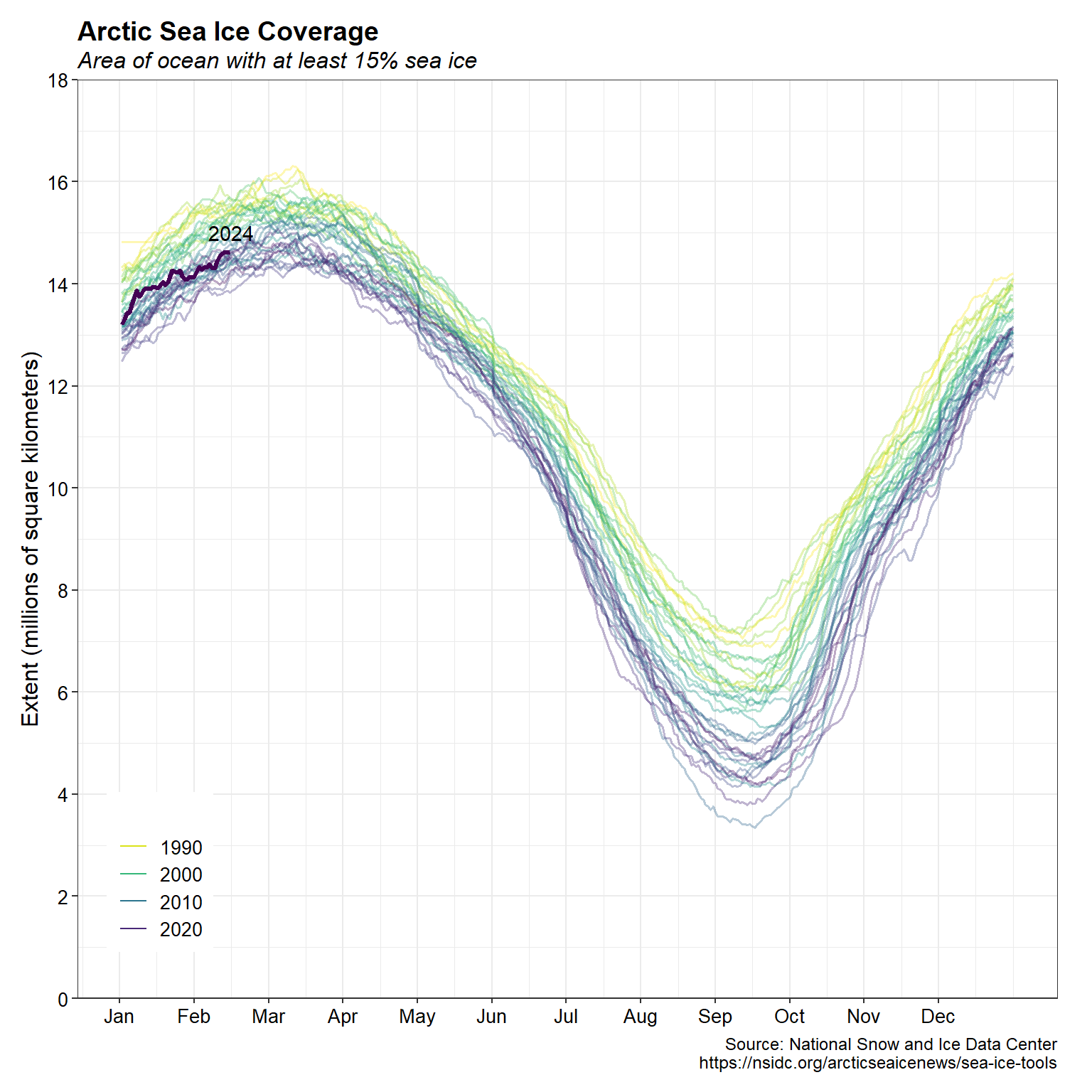
Shown below are up-to-date satellite observations of sea ice extent in the Arctic, along with comparisons with the historical satellite record of more than 4 decades. The plot shows daily ASIE, in millions of square kilometers, color coded by year in a sequential fashion. The color scheme moves from yellow to purple, from 1988 to 2023, respectively; daily values for January through 14 February 2024 is shown as a thick dark purple line segent.
Sea ice extent in the Arctic grows throughout the winter, before peaking in March. Melting occurs during the spring as the sun gets stronger, and in September the extent of the ice cover is typically only around one third of its winter maximum. These results illustrate the general decrease in Arctic sea ice coverage over the last 4 decades.
# Create caption
cap <- paste0(
  'Source: National Snow and Ice Data Center\n',
  'https://nsidc.org/arcticseaicenews/sea-ice-tools'
)

# Plot sea ice extent for all years
seaice %>%
  mutate(latestyear = as.factor((year == max(year)))) %>%
  ggplot(aes(x = monthday, y = extent, group = year, color = year,
         alpha = latestyear)) +
  geom_line(aes(linewidth = latestyear)) +
  scale_alpha_manual(values = c('FALSE' = 0.35, 'TRUE' = 1), guide = 'none') +
  scale_color_viridis("", direction = -1, guide = guide_legend(reverse = FALSE))  +
  scale_linewidth_manual(values = c('FALSE' = 0.6, 'TRUE' = 1.2), guide = 'none') +
  scale_x_continuous(breaks = 1:12, labels = mon) +
  scale_y_continuous(limits = c(0, 18),
                     breaks = seq(0, 18, by = 2),
                     expand = c(0, 0)) +
  annotate('text', x = 2.5, y = 15, label = max(seaice$year)) +
  labs(title = 'Arctic Sea Ice Coverage',
       subtitle = 'Area of ocean with at least 15% sea ice',
       caption = cap,
       x = NULL,
       y = 'Extent (millions of square kilometers)') +
   theme_bw() +
   my_theme +
   theme(legend.key.height = unit(1, 'line'),
         legend.text = element_text(size = 10))
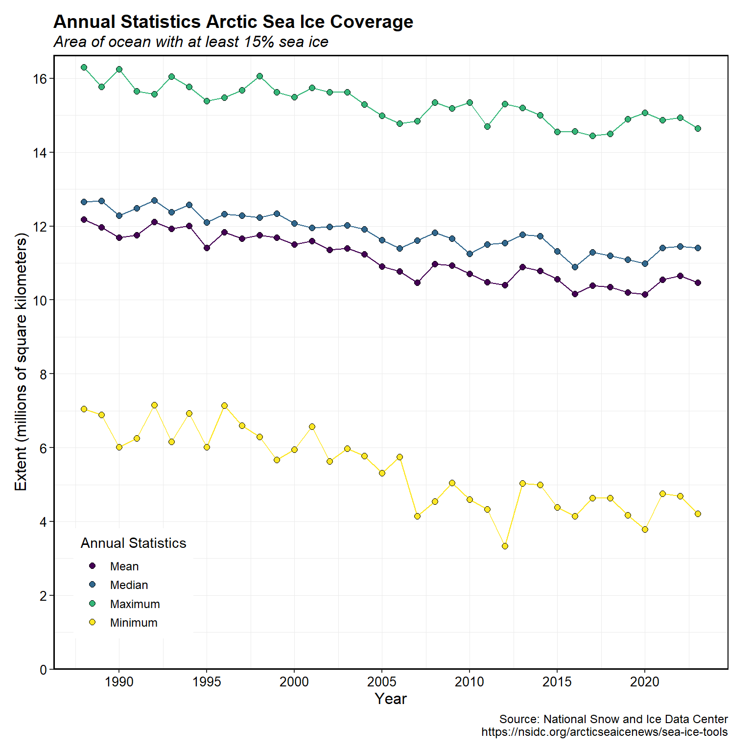
A plot of the minimum, maximum, mean, and median annual ASIE from 1988 through 2023 is shown below. The ASIE is extremely variable, both seasonally and from year to year. Higher year-to-year variability in the data appears associated with the summer months where sea ice extent is at a minimum. The plots suggests a downward trend in ASIE starting at the beginning of the dataset in 1988 and extending to 2015, after which, there is much less of a decrease, if any.
# Get data
seaice2 <- seaice %>%
  filter(year != 2024) %>%
  dplyr::select(date, extent) %>%
  rename(Date = date, Value = extent)

# Plot of annual statistics
plot_annual_stats(
  data = seaice2,
  start_year = 1988,
  end_year = 2023
)[[1]] +
  labs(title = 'Annual Statistics Arctic Sea Ice Coverage',
       subtitle = 'Area of ocean with at least 15% sea ice',
       caption = cap,
       y = 'Extent (millions of square kilometers)') +
  my_theme +
  theme(legend.key.height = unit(1, 'line'))
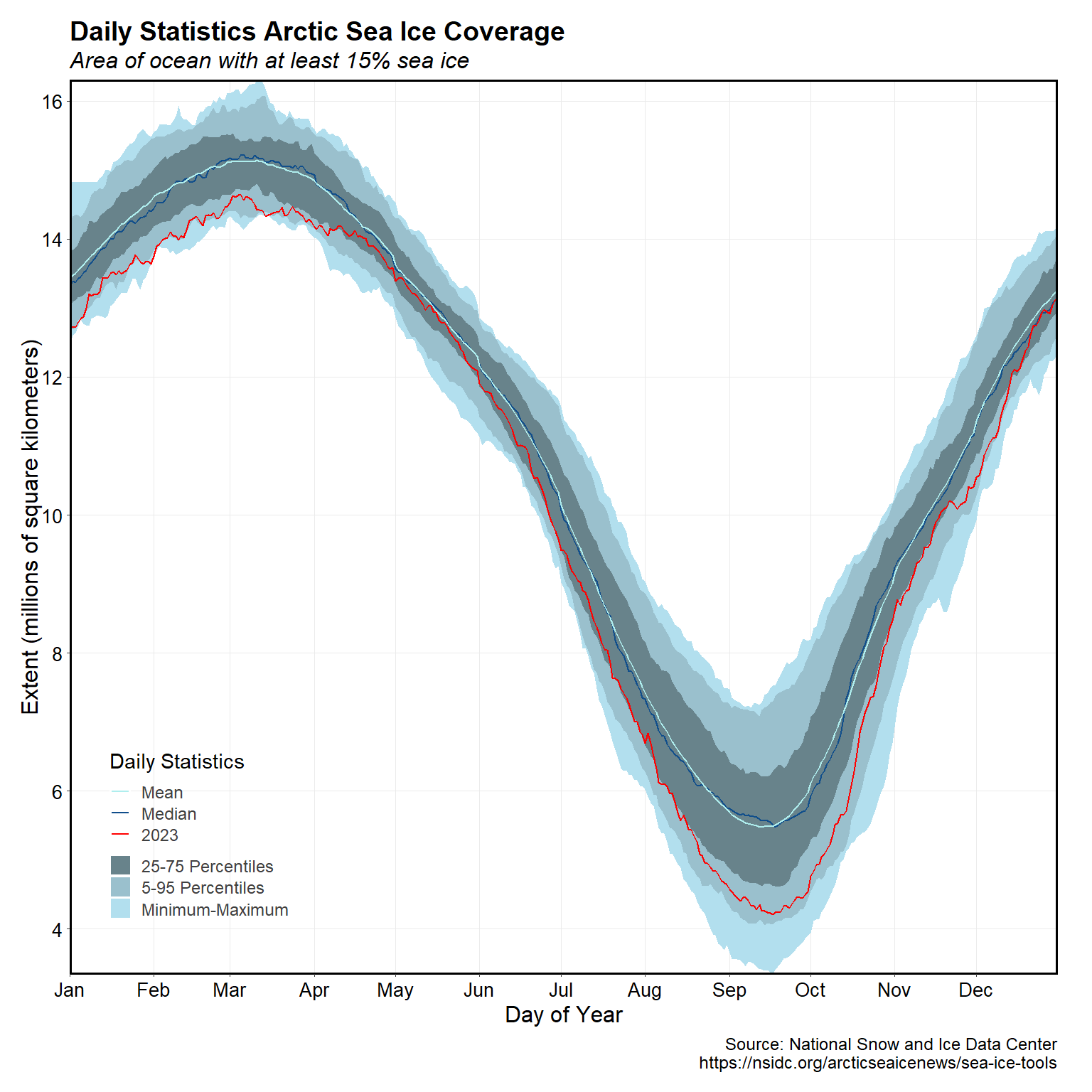
The plot below shows the mean and median ASIE from 1988 through 2023, along with the more recent data in 2023 for comparison. The blue areas around the mean line show the inner percentiles (25th to 75th percentiles), the outer percentiles (5th to 95th percentiles), and the minimum and maximum values of the data. The 2023 data generally fall outside the inner percentiles but within the outer percentiles.
# Plot of daily mean, median, min, and max values with inner and outer percentiles
plot_daily_stats(
  data = seaice2,
  start_year = 1988,
  end_year = 2023,
  log_discharge = FALSE,
  add_year = 2023
)[[1]] +
  labs(title = 'Daily Statistics Arctic Sea Ice Coverage',
       subtitle = 'Area of ocean with at least 15% sea ice',
       caption = cap,
       y = 'Extent (millions of square kilometers)') +
  my_theme
Monthly
Summary statistics of ASIE by month are tabulated below for all years starting in 1988.
# Calculate monthly stats
calc_longterm_daily_stats(data = seaice2, dates = Date)
## # A tibble: 13 × 7
##    Month      Mean Median Maximum Minimum   P10   P90
##    <fct>     <dbl>  <dbl>   <dbl>   <dbl> <dbl> <dbl>
##  1 Jan       14.0   14.0    15.6    12.5  13.2  14.9
##  2 Feb       14.9   14.9    16.1    13.8  14.2  15.6
##  3 Mar       15.0   15.1    16.3    14.1  14.4  15.6
##  4 Apr       14.3   14.3    15.6    12.9  13.6  15.1
##  5 May       12.9   13.0    14.4    11.1  12.2  13.7
##  6 Jun       11.3   11.4    12.9     9.23 10.2  12.3
##  7 Jul        8.77   8.83   11.4     6.03  7.16 10.3
##  8 Aug        6.46   6.46    8.93    3.65  5.00  7.90
##  9 Sep        5.62   5.64    8.21    3.34  4.30  7.10
## 10 Oct        7.53   7.69   10.2     4.11  5.43  9.36
## 11 Nov       10.2   10.2    12.5     7.22  8.99 11.3
## 12 Dec       12.5   12.5    14.2    10.2  11.4  13.5
## 13 Long-term 11.1   11.9    16.3     3.34  6.07 15.0
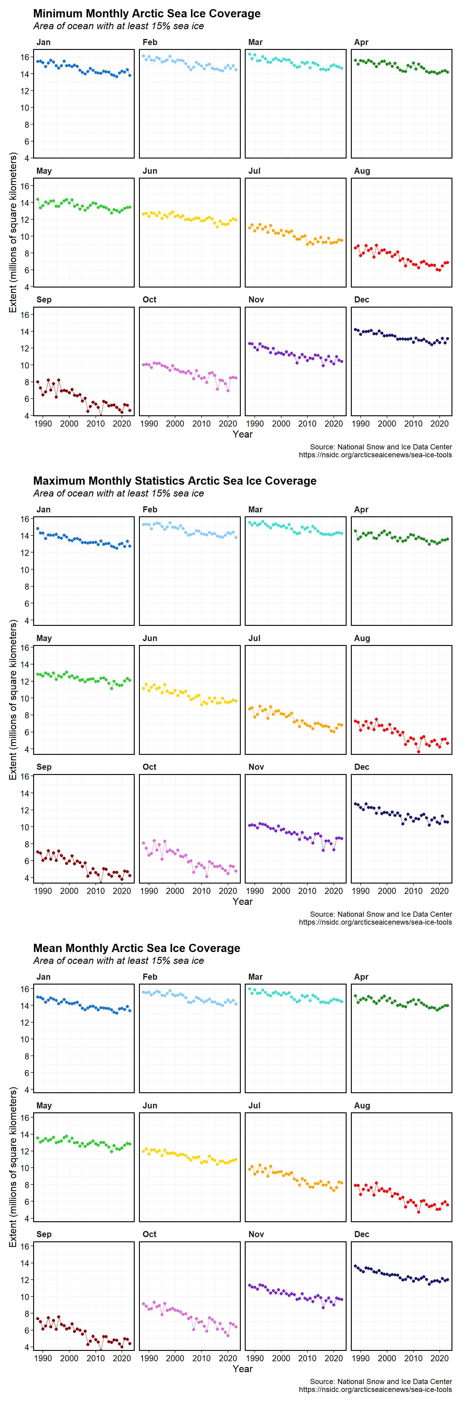
Plots of the monthly minimum, maximum, and mean ASIE are shown below. ASIE declines in all months with larger variability occurring in August through October when the ice extent is at a minimum.
# Plot of minimum monthly statistics
p1 <- plot_monthly_stats(
  data = seaice2,
  start_year = 1988,
  end_year = 2023
)[[3]] +
  scale_x_continuous(limits = c(1988, 2023),
                     breaks = seq(1990, 2023, by = 10)) +
  labs(title = 'Minimum Monthly Arctic Sea Ice Coverage',
       subtitle = 'Area of ocean with at least 15% sea ice',
       caption = cap,
       y = 'Extent (millions of square kilometers)') +
  my_theme

# Plot of maximim monthly statistics
p2 <- plot_monthly_stats(
  data = seaice2,
  start_year = 1988,
  end_year = 2023
)[[4]] +
  scale_x_continuous(limits = c(1988, 2023),
                     breaks = seq(1990, 2023, by = 10)) +
  labs(title = 'Maximum Monthly Statistics Arctic Sea Ice Coverage',
       subtitle = 'Area of ocean with at least 15% sea ice',
       caption = cap,
       y = 'Extent (millions of square kilometers)') +
  my_theme

# Plot of mean monthly statistics
p3 <- plot_monthly_stats(
  data = seaice2,
  start_year = 1988,
  end_year = 2023
)[[1]] +
  scale_x_continuous(limits = c(1988, 2023),
                     breaks = seq(1990, 2023, by = 10)) +
  labs(title = 'Mean Monthly Arctic Sea Ice Coverage',
       subtitle = 'Area of ocean with at least 15% sea ice',
       caption = cap,
       y = 'Extent (millions of square kilometers)') +
  my_theme

# Show all plots
gridExtra::grid.arrange(p1, p2, p3, ncol = 1)
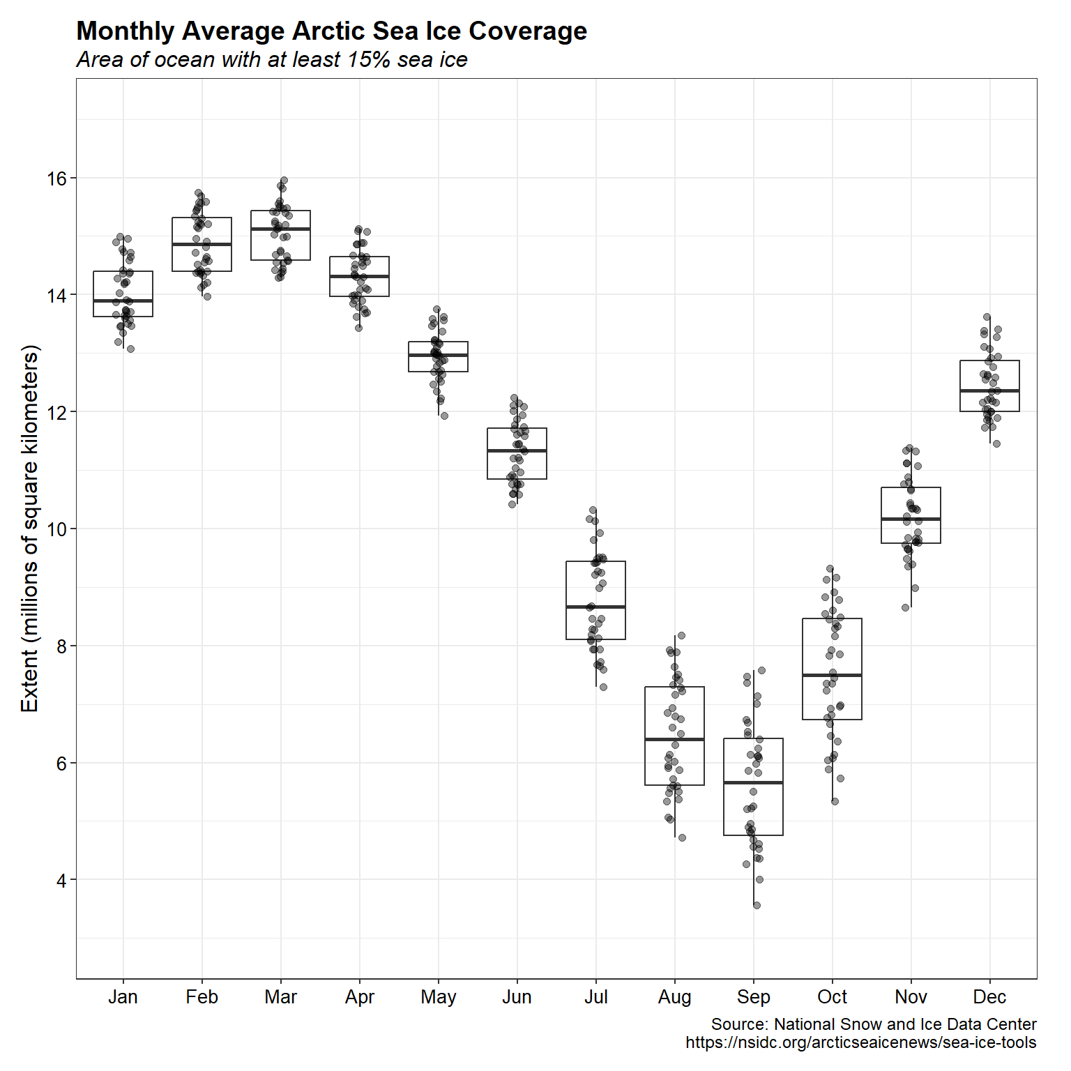
Box plots of monthly average ASIE from 1988 through 2023 are shown below. Individual monthly averages for each year are included on the plot as grey circles. The data further illustrate higher variability occurring during August through October, when ASIE is at a minimum.
# Get monthly statistics
cdat <- seaice %>%
  filter(year != 2024) %>%
  group_by(month, year) %>%
  summarize(
    exmean = mean(extent, na.rm = TRUE),
    exmin = min(extent, na.rm = TRUE),
    exmax = max(extent, na.rm = TRUE)
  ) %>%
  ungroup() %>%
  data.frame()

# Create boxplot
jitterer <- position_jitter(seed = 123, width = 0.1, height = 0)
ggplot(data = cdat, aes(x = month, y = exmean)) +
  geom_boxplot(coef = 10^16, outlier.shape = NA, outlier.size = 0,
               notch = FALSE, fill = NA) +
  geom_point(size = 1.6, alpha = 0.4, position = jitterer) +
  scale_y_continuous(limits = c(3, 17),
                     breaks = seq(4, 16, by = 2)) +
  labs(title = 'Monthly Average Arctic Sea Ice Coverage',
       subtitle = 'Area of ocean with at least 15% sea ice',
       caption = cap,
       x = NULL,
       y = 'Extent (millions of square kilometers)') +
  theme_bw() +
  my_theme
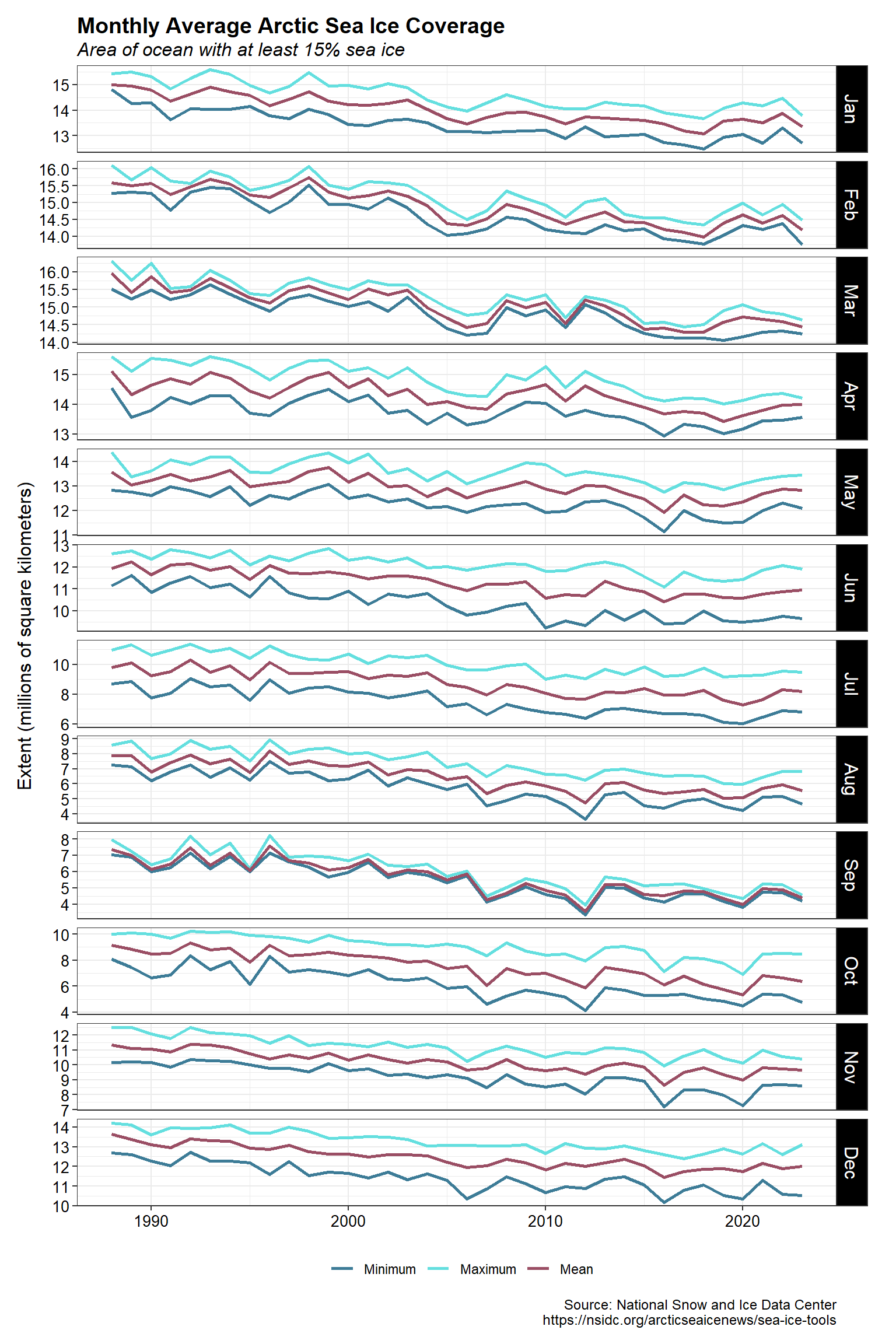
Line plots of the monthly minimum, maximum, and mean ASIE are shown below, where each color corresponds to a different statistic. The extent of sea ice changes throughout the seasons, with the smallest and largest extents occurring in summer and winter, respectively. Starting at the beginning of the dataset in 1988, ASIE declines until about 2015. A decline in ASIE is not evident after about 2015.
# Plot monthly min, max, and mean
cdat %>%
  gather(key = 'param', value = 'extent', 3:5) %>%
  mutate(param = factor(
    param,
    levels = c('exmin', 'exmax', 'exmean'))
  ) %>%
  ggplot(aes(x = year, y = extent, color = param)) +
  geom_line(linewidth = 1) +
  facet_grid(month ~ ., scales = 'free_y') +
  labs(title = 'Monthly Average Arctic Sea Ice Coverage',
       subtitle = 'Area of ocean with at least 15% sea ice',
       caption = cap,
       x = NULL,
       y = 'Extent (millions of square kilometers)') +
  scale_color_manual(name = NULL,
                     values = c('exmin'  = '#3D7C97',
                                'exmax'  = '#64DFDF',
                                'exmean' = '#9A4E64'),
                     labels = c('exmin'  = 'Minimum',
                                'exmax'  = 'Maximum',
                                'exmean' = 'Mean')) +
  theme_bw() +
  my_theme +
  theme(legend.position = 'bottom',
        legend.justification = 'center',
        strip.background  = element_rect(fill = 'black'),
        strip.text = element_text(size = 12, color = 'white'))
Extremes
Another way to assess the changes in ASIE, complementary to trend analysis, is to examine the occurrences and frequency of record high and record low ice extent values. Although these extreme events may vary in timing and duration, taken together, they are an indicator of rapid change in ASIE.
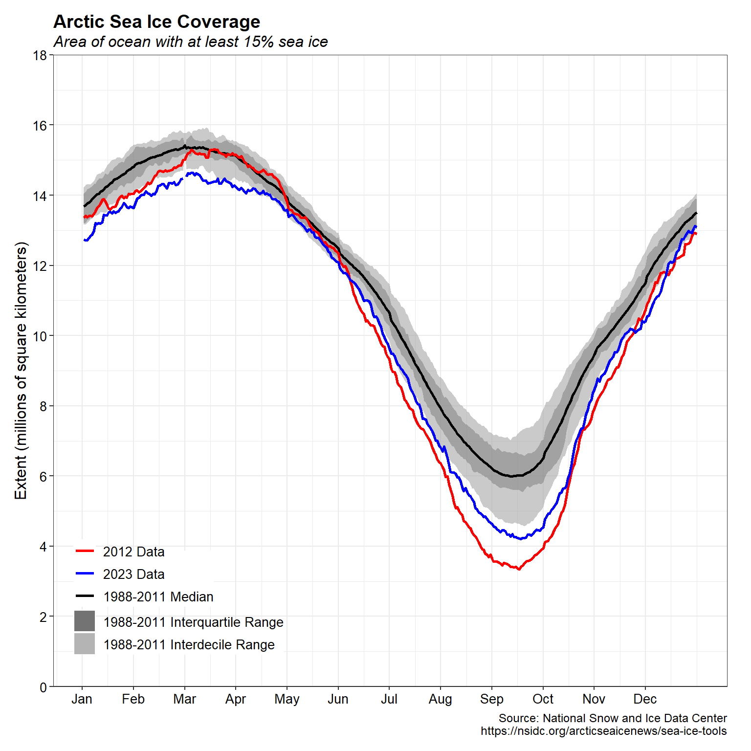
The plot below shows the median ASIE from 1988 through 2011, along with the record low data in 2012 and the more recent data in 2023. The gray areas around the median line show the interquartile and interdecile ranges of the 1988-2011 data. ASIE in August through November of 2012 and 2023 lie outside the interquartile and interdecile ranges.
# Prep data to get 1988-2011 median, IQR, and IDR; then add 2012 and 2023 data
seaice3 <- seaice %>%
  filter(year < 2012) %>%
  group_by(month, day, monthday) %>%
  summarize(
    med = mean(extent),
    Q1 = quantile(extent, 0.25, names = F),
    Q3 = quantile(extent, 0.75, names = F),
    P1 = quantile(extent, probs = 0.1, names = F),
    P9 = quantile(extent, probs = 0.9, names = F)
  ) %>%
  ungroup() %>%
  left_join(
    seaice %>%
      filter(year == 2012) %>%
      group_by(month, day, monthday) %>%
      summarize(med12 = mean(extent)) %>%
      ungroup(),
    by = c('month', 'day', 'monthday')
  ) %>%
  left_join(
    seaice %>%
      filter(year == 2023) %>%
      group_by(month, day, monthday) %>%
      summarize(med23 = mean(extent)) %>%
      ungroup(),
    by = c('month', 'day', 'monthday')
  )

# Plot sea ice extent for 1988-2011 median, IQR, and IDR; and separately for 2012 and 2023
ggplot(data = seaice3) +
  geom_ribbon(aes(x = monthday, ymin = Q1, ymax = Q3, fill = 'D4'),
              alpha = 0.6) +
  geom_ribbon(aes(x = monthday, ymin = P1, ymax = P9, fill = 'D5'),
              alpha = 0.6) +
  geom_line(aes(x = monthday, y = med, color = 'D3'), linewidth = 1) +
  geom_line(aes(x = monthday, y = med12, color = 'D1'), linewidth = 1) +
  geom_line(aes(x = monthday, y = med23, color = 'D2'), linewidth = 1) +
  scale_x_continuous(breaks = 1:12, labels = mon) +
  scale_y_continuous(limits = c(0, 18),
                     breaks = seq(0, 18, by = 2),
                     expand = c(0, 0)) +
  scale_color_manual(name = NULL,
                     values = c('D1' = 'red',
                                'D2' = 'blue',
                                'D3' = 'black'),
                     labels = c('D1' = '2012 Data',
                                'D2' = '2023 Data',
                                'D3' = '1988-2011 Median')) +
  scale_fill_manual(name = NULL,
                    values = c('D4' = 'grey35',
                               'D5' = 'grey65'),
                    labels = c('D4' = '1988-2011 Interquartile Range',
                               'D5' = '1988-2011 Interdecile Range')) +
  labs(title = 'Arctic Sea Ice Coverage',
       subtitle = 'Area of ocean with at least 15% sea ice',
       caption = cap,
       x = NULL,
       y = 'Extent (millions of square kilometers)') +
   theme_bw() +
   my_theme +
   theme(legend.text = element_text(size = 10),
         legend.margin = margin(-0.5, 0, 0, 0, unit = 'cm'))
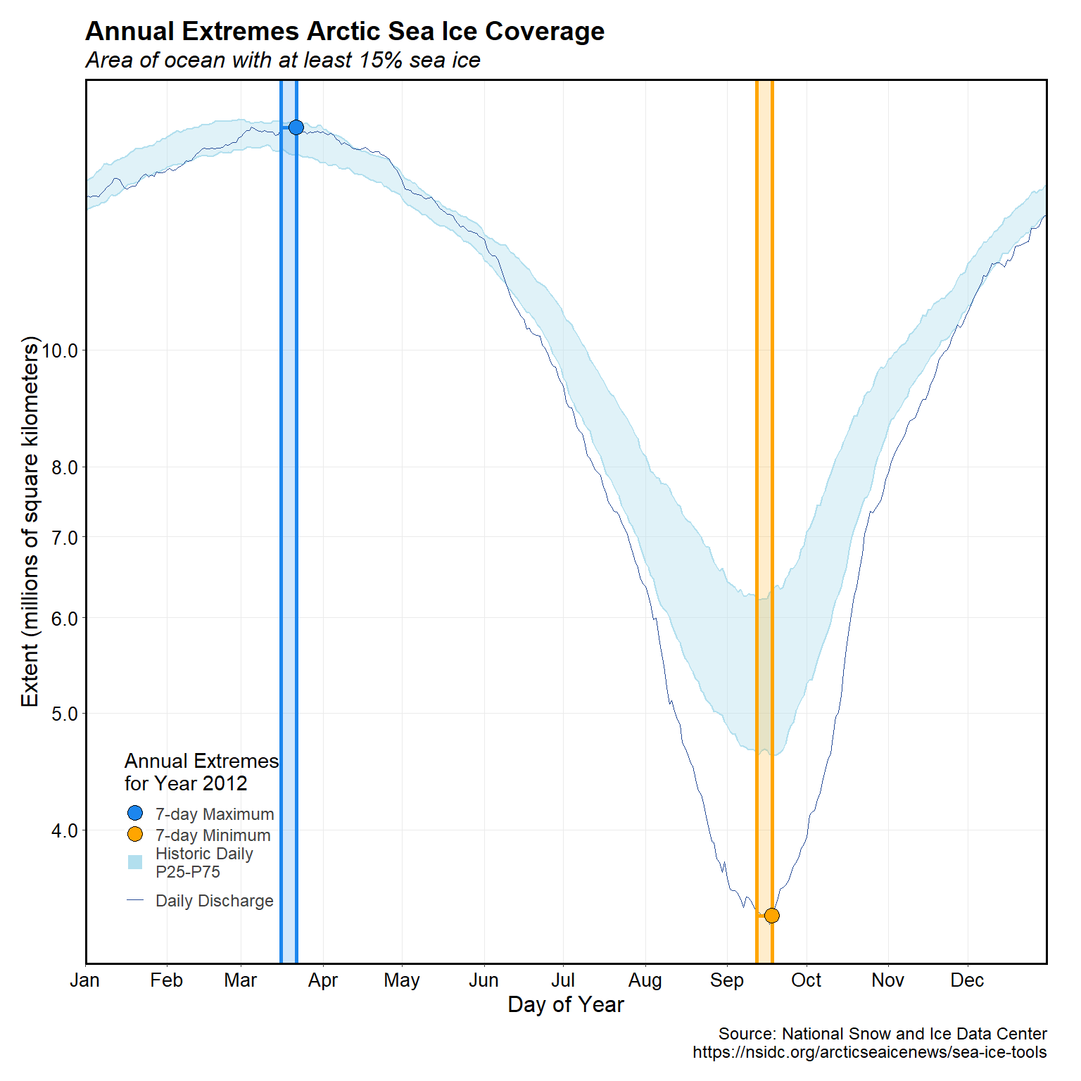
The daily ASIE for the record low year of 2012 is shown below. Also included in the plot are the values and timing of annual 7-day low and high values, and the normal range, defined as between the 25th and 75th percentiles. The 2012 record-breaking minimum has be attributed to an abnormally thin, vulnerable ice cover whose reduction was accelerated by an intense but brief storm (Zhang et al. 2013).
# Plot of annual high and low sea ice extent for a specific year
plot_annual_extremes_year(
  data = seaice2,
  roll_days_min = 7,
  roll_days_max = 7,
  start_year = 1988,
  year_to_plot = 2012
)[[1]] +
  labs(title = 'Annual Extremes Arctic Sea Ice Coverage',
       subtitle = 'Area of ocean with at least 15% sea ice',
       caption = cap,
       y = 'Extent (millions of square kilometers)') +
  my_theme
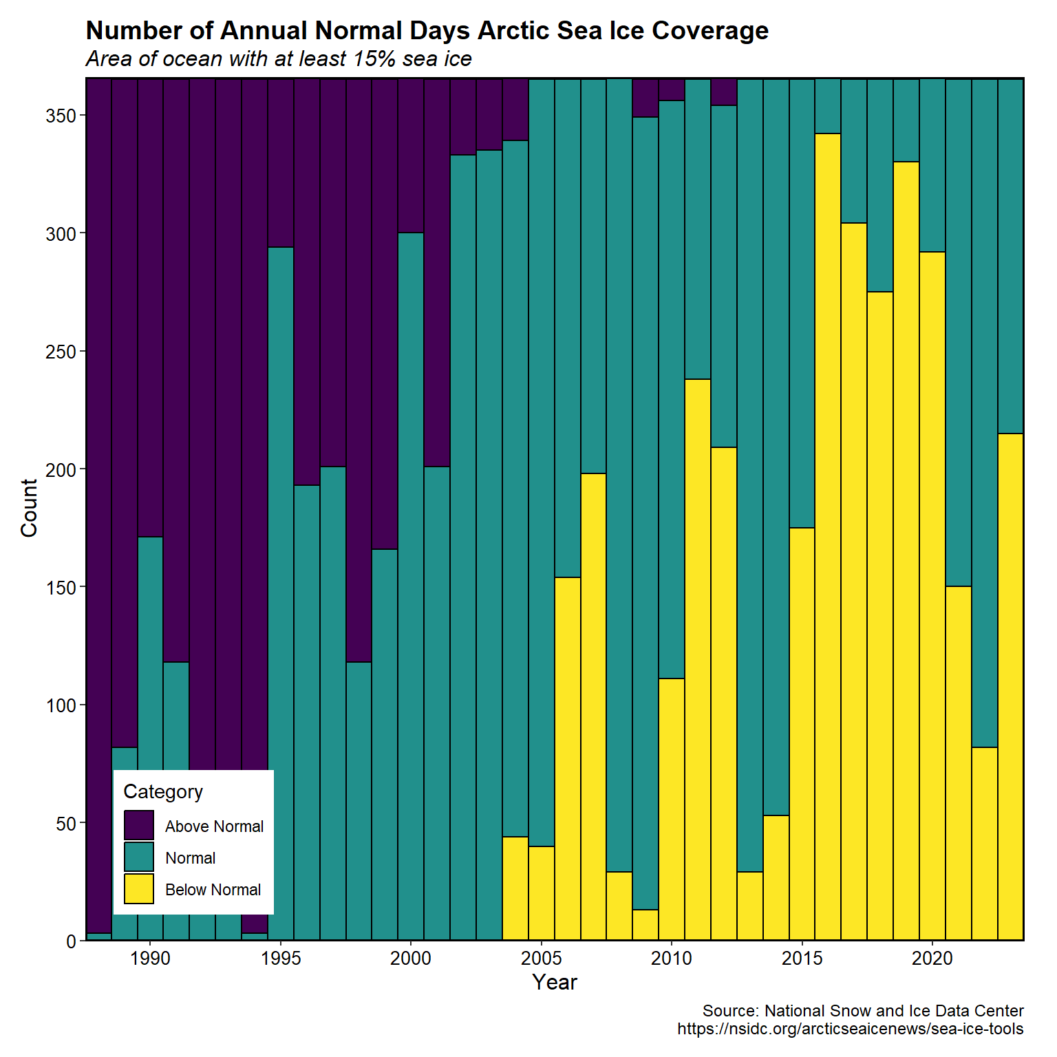
A plot of the number of days per year within, above, and below the normal range (between the 25th and 75th percentiles) for each day of the year is shown below. The normal range is calculated for each day of the year from all years. Starting in 2004, the number of days each year that is below the normal range increases.
# Bar plot of annual count of normal days and days above and below normal
plot_annual_normal_days(
  data = seaice2,
  start_year = 1988
)[[1]] +
  labs(title = 'Number of Annual Normal Days Arctic Sea Ice Coverage',
       subtitle = 'Area of ocean with at least 15% sea ice',
       caption = cap,
       y = 'Count') +
  my_theme +
  theme(legend.position = c(0.03, 0.03))
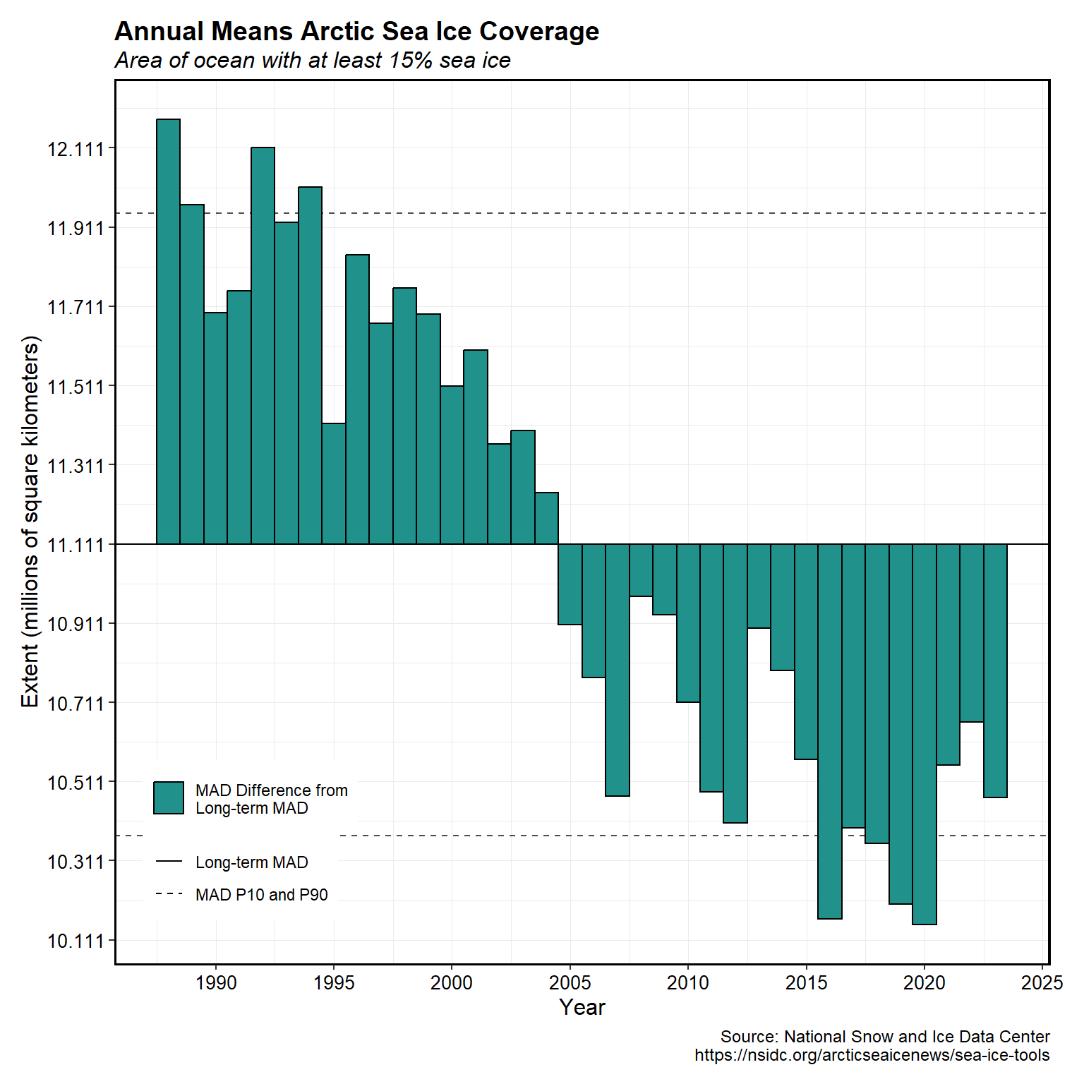
A plot of the annual means compared to the long-term annual mean as a point of reference is shown below. The x-axis is located at the long-term mean annual datum (mean of all values over all years) and the bars show the annual means. The plot is essentially an anomaly plot but with the y-value corresponding to the mean value and not the difference from the log-term annual mean. Similar to the number of days each year below normal, there is an overall decrease in the annual mean ASIE starting in 2004.
# Plot of annual means compared to long-term mean
plot_annual_means(
  data = seaice2,
  start_year = 1974
)[[1]] +
  labs(title = 'Annual Means Arctic Sea Ice Coverage',
       subtitle = 'Area of ocean with at least 15% sea ice',
       caption = cap,
       y = 'Extent (millions of square kilometers)') +
  my_theme
Trend Analysis
Mann-Kendall Test
Trend analysis using the Mann-Kendall test (Mann 1945; Kendall 1975) was performed on monthly ASIE for 1988 through 2023. The Mann-Kendall test is a nonparametric procedure used to assess whether there is an upward or downward monotonic trend in the variable of interest over time. The test evaluates each set of data values as an ordered time series where each value is compared to all subsequent values. The tabulated results shown below indicate a strong decreasing trend in ASIE for all months between 1988 and 2023.
# MK trend analysis on monthly data from 1998 through 2023
library(Kendall)
cdat %>%
  arrange(month, year) %>%
  group_by(month) %>%
  summarize(
    Obs    = length(exmean),
    Min    = min(exmean, na.rm = TRUE),
    Max    = max(exmean, na.rm = TRUE),
    Mean   = mean(exmean, na.rm = TRUE),
    Median = median(exmean, na.rm = TRUE),
    SD     = round(sd(exmean, na.rm = TRUE), 3),
    CV     = round(SD/Mean, 3),
    S      = MannKendall(exmean)$S,
    pval   = 0.5*MannKendall(exmean)$sl,
    Trend  = ifelse(pval < 0.05, ifelse(S > 0, 'Increasing', 'Decreasing'), 'No Trend')
  ) %>%
  ungroup() %>%
  mutate_at(3:6, round, 2) %>%
  data.frame()
##    month Obs   Min   Max  Mean Median    SD    CV    S         pval      Trend
## 1    Jan  36 13.08 14.99 14.02  13.90 0.534 0.038 -464 1.427317e-10 Decreasing
## 2    Feb  36 13.97 15.75 14.88  14.86 0.521 0.035 -422 4.893005e-09 Decreasing
## 3    Mar  36 14.29 15.96 15.05  15.13 0.485 0.032 -394 4.325114e-08 Decreasing
## 4    Apr  36 13.43 15.12 14.31  14.31 0.460 0.032 -356 6.643332e-07 Decreasing
## 5    May  36 11.92 13.75 12.95  12.97 0.429 0.033 -346 1.305857e-06 Decreasing
## 6    Jun  36 10.41 12.24 11.31  11.34 0.528 0.047 -434 1.841372e-09 Decreasing
## 7    Jul  36  7.29 10.32  8.77   8.66 0.837 0.095 -420 5.744011e-09 Decreasing
## 8    Aug  36  4.72  8.18  6.46   6.40 0.959 0.148 -424 4.165068e-09 Decreasing
## 9    Sep  36  3.57  7.58  5.62   5.67 1.070 0.190 -418 6.738157e-09 Decreasing
## 10   Oct  36  5.33  9.32  7.53   7.50 1.105 0.147 -460 2.026272e-10 Decreasing
## 11   Nov  36  8.66 11.38 10.20  10.17 0.677 0.066 -444 7.994715e-10 Decreasing
## 12   Dec  36 11.46 13.63 12.45  12.36 0.560 0.045 -484 2.369836e-11 Decreasing
Trend analysis also was performed on monthly ASIE using data from 2010 through 2023. The tabulated results shown below indicate no discernible trend in ASIE for all months, except, April, between 2010 and 2023. For the month of April, ASIE exhibits a decreasing trend.
# MK trend analysis on monthly data from 2016 through 2023
library(Kendall)
cdat %>%
  filter(year > 2010) %>%
  arrange(month, year) %>%
  group_by(month) %>%
  summarize(
    Obs    = length(exmean),
    Min    = min(exmean, na.rm = TRUE),
    Max    = max(exmean, na.rm = TRUE),
    Mean   = mean(exmean, na.rm = TRUE),
    Median = median(exmean, na.rm = TRUE),
    SD     = round(sd(exmean, na.rm = TRUE), 3),
    CV     = round(SD/Mean, 3),
    S      = MannKendall(exmean)$S,
    pval   = 0.5*MannKendall(exmean)$sl,
    Trend  = ifelse(pval < 0.05, ifelse(S > 0, 'Increasing', 'Decreasing'), 'No Trend')
  ) %>%
  ungroup() %>%
  mutate_at(3:6, round, 2) %>%
  data.frame()
##    month Obs   Min   Max  Mean Median    SD    CV   S       pval      Trend
## 1    Jan  13 13.08 13.87 13.52  13.57 0.220 0.016 -16 0.18006080   No Trend
## 2    Feb  13 13.97 14.72 14.38  14.39 0.221 0.015 -14 0.21385527   No Trend
## 3    Mar  13 14.29 15.20 14.61  14.57 0.273 0.019 -14 0.21385527   No Trend
## 4    Apr  13 13.43 14.63 13.92  13.89 0.315 0.023 -28 0.04975436 Decreasing
## 5    May  13 11.92 13.01 12.58  12.68 0.333 0.026  -8 0.33466703   No Trend
## 6    Jun  13 10.41 11.36 10.80  10.77 0.235 0.022   0 0.50000000   No Trend
## 7    Jul  13  7.29  8.38  7.94   7.94 0.328 0.041   2 0.47567606   No Trend
## 8    Aug  13  4.72  6.08  5.52   5.57 0.398 0.072   4 0.42738855   No Trend
## 9    Sep  13  3.57  5.22  4.61   4.62 0.465 0.101  -4 0.42738855   No Trend
## 10   Oct  13  5.33  7.45  6.45   6.46 0.611 0.095 -18 0.14983270   No Trend
## 11   Nov  13  8.66 10.11  9.58   9.73 0.405 0.042 -14 0.21385527   No Trend
## 12   Dec  13 11.46 12.35 11.96  12.00 0.234 0.020 -18 0.14983270   No Trend
Theil-Sen Regression
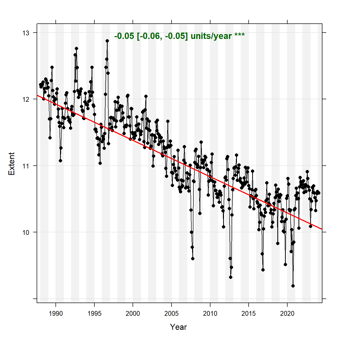
Theil-Sen regression (Sen 1968; Theil 1950) was conducted on daily ASIE. This procedure is a generalized median-based regressor that calculates slopes of all possible combinations of sample points. Consequently, the Theil-Sen line estimates the change in median concentration over time and not the mean as in linear regression. When the explanatory variable is a measure of time, the significance test for the slope is a test for (temporal) trend.
Theil-Sen regression was first conducted using all daily ASIE values between 1988 and 2023. For this case, the data were deseasoned using STL (seasonal trend decomposition using loess) (Cleveland et al. 1990) prior to regression. The STL method uses locally fitted regression models to decompose a time series into trend, seasonal, and remainder components. STL provides meaningful results only if a recurring temporal pattern exists in the data. The results of the Theil-Sen regression analysis are shown below and indicate a strong decreasing trend in ASIE between 1988 and 2023.
# Load library
library(openair)

# Select variables
seaice_ts <- seaice %>% dplyr::select(date, extent)

# Theil-Sen slope estimates and tests for trend

# Slope estimates using the function stl (seasonal trend decomposition using
# loess) to deseason data first
TheilSen(
  seaice_ts,
  pollutant = 'extent',
  type = 'default',
  deseason = TRUE,
  date.format = '%Y',
  xlab = 'Year',
  ylab = 'Extent',
  lab.cex = 1.1,
  lab.frac = 0.97,
  data.col = 'black', pch = 16, cex = 0.8,
  trend = list(lty = c(1, 1), lwd = c(2, 0), col = c('red', NA))
)
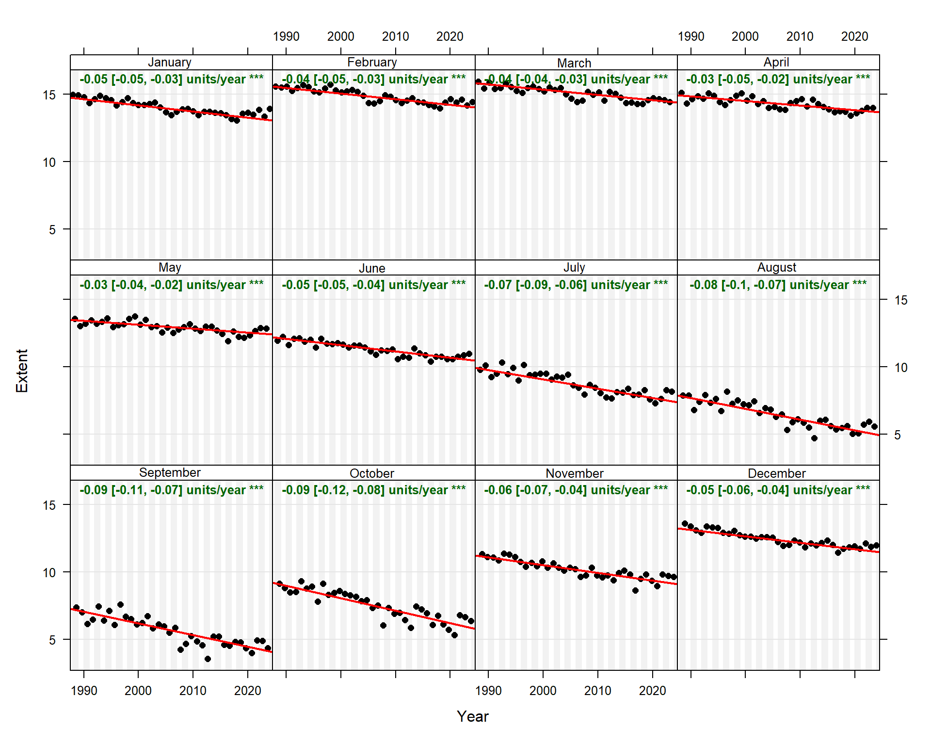
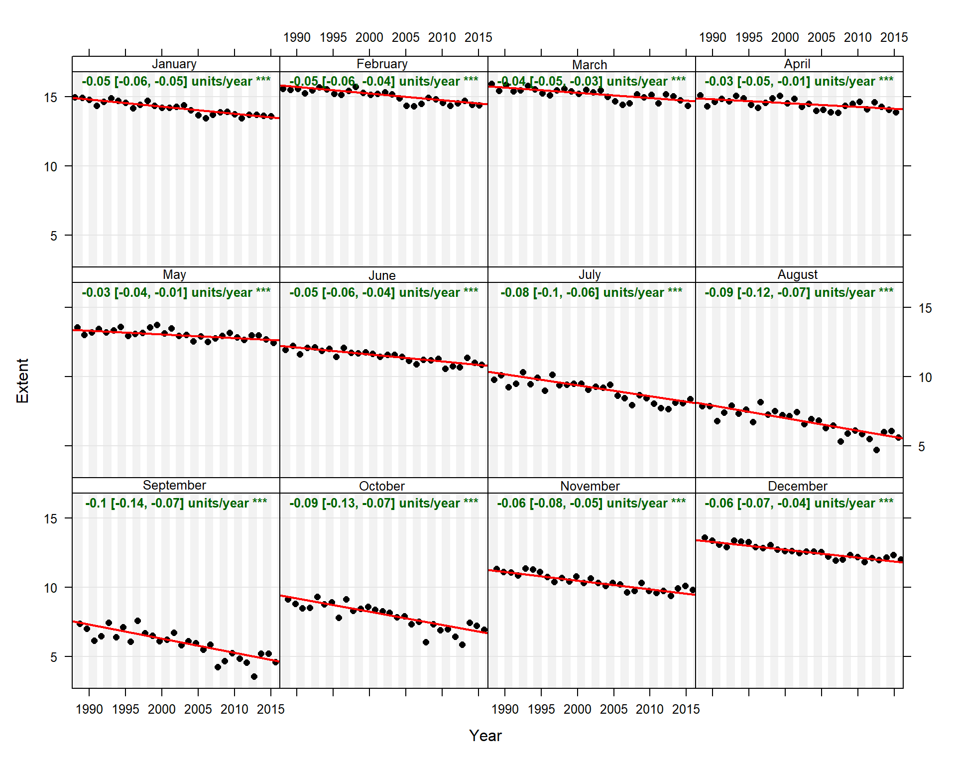
Theil-Sen regression was conducted by month using ASIE values between 1988 and 2023. The results are shown below and indicate statistically significant decreasing trends of ASIE in all months, with the largest decreasing trend observed for September and October.
# Slope estimates by month for all years
TheilSen(
  seaice_ts,
  pollutant = 'extent',
  type = 'month',
  deseason = FALSE,
  date.format = '%Y',
  xlab = 'Year',
  ylab = 'Extent',
  y.relation = 'same',
#  y.relation = 'free',
  date.breaks = 4,
  lab.cex = 0.8,
  lab.frac = 0.98,
  data.col = 'black', pch = 16, cex = 0.8,
  trend = list(lty = c(1, 1), lwd = c(2, 0), col = c('red', NA))
)
Theil-Sen regression was conducted by month using ASIE values between 1988 and 2015. The results are shown below and indicate statistically significant decreasing trends of ASIE in all months, with the largest decreasing trend observed for September.
# Slope estimates by month for years 1988-2015
TheilSen(
  selectByDate(seaice_ts, year = 1988:2015),
  pollutant = 'extent',
  type = 'month',
  deseason = FALSE,
  date.format = '%Y',
  xlab = 'Year',
  ylab = 'Extent',
  y.relation = 'same',
#  y.relation = 'free',
  date.breaks = 4,
  lab.cex = 0.8,
  lab.frac = 0.98,
  data.col = 'black', pch = 16, cex = 0.8,
  trend = list(lty = c(1, 1), lwd = c(2, 0), col = c('red', NA))
)
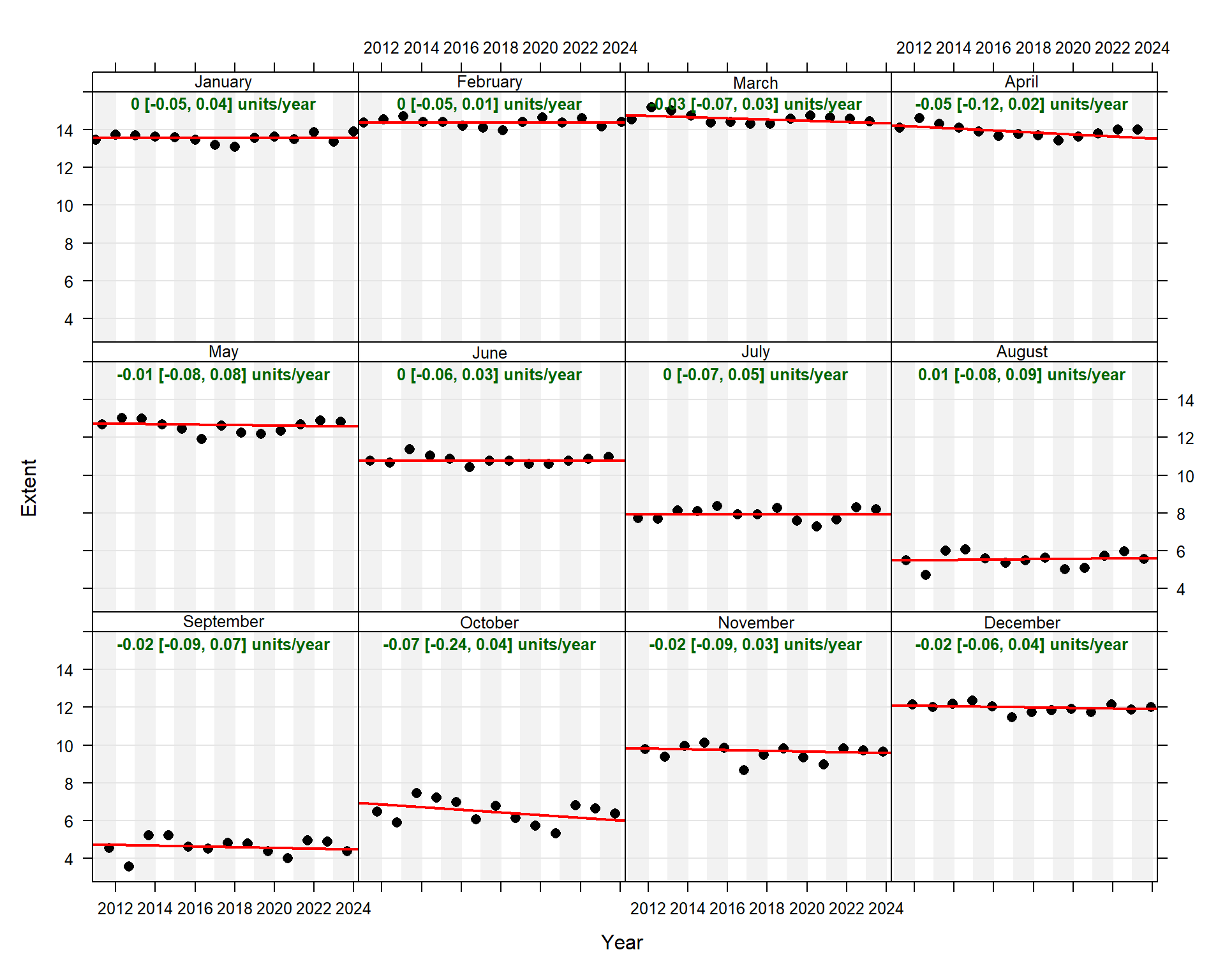
Theil-Sen regression was conducted by month using ASIE values between 2011 and 2023. The results are shown below and indicate no discernable trends (slope is not statistically different than 0).
# Slope estimates by month for years 2011-2023
TheilSen(
  filter(seaice_ts, format(date, '%Y') > 2010),
  pollutant = 'extent',
  type = 'month',
  deseason = FALSE,
  date.format = '%Y',
  xlab = 'Year',
  ylab = 'Extent',
  y.relation = 'same',
#  y.relation = 'free',
  date.breaks = 4,
  lab.cex = 0.8,
  lab.frac = 0.98,
  data.col = 'black', pch = 16, cex = 1,
  trend = list(lty = c(1, 1), lwd = c(2, 0), col = c('red', NA))
)
Time Series Analysis
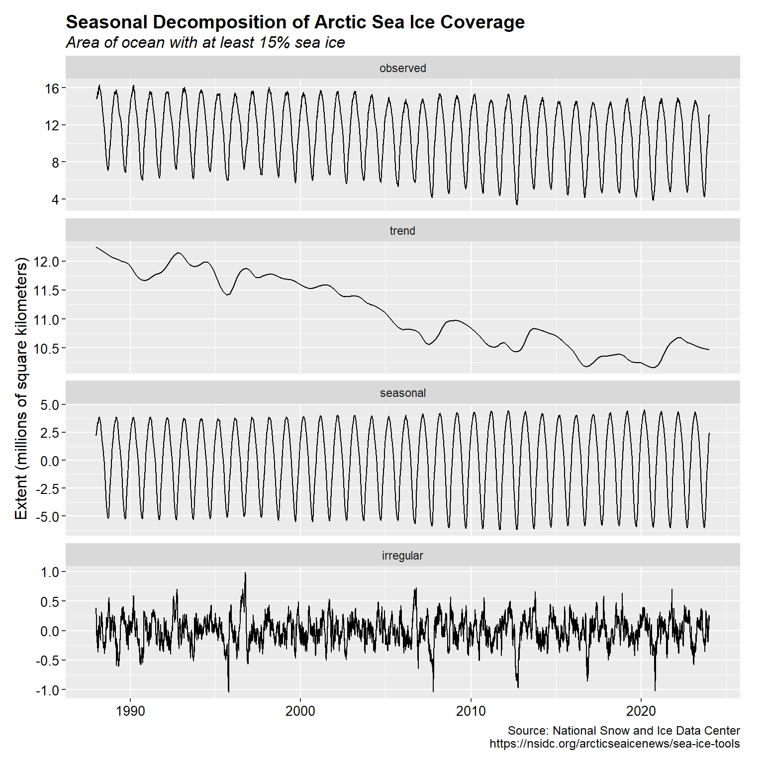
An exploratory analysis of the ASIE time series data was performed. A seasonal decomposition of the data is shown below and consists of four plots: observed, trend, seasonal and random components. This visualization was created using the ggseas package that integrates into a ggplot2 graphic workflow.
# Create subset of data by removing 2024
seaice_sub <- seaice %>%
  filter(year < 2024)

# Visualize decomposition of data
ggsdc(data = seaice_sub, aes(x = date, y = extent), method = 'stl',
      s.window = 7, frequency = 365.25) +
  geom_line() +
  labs(title = 'Seasonal Decomposition of Arctic Sea Ice Coverage',
       subtitle = 'Area of ocean with at least 15% sea ice',
       caption = cap,
       x = NULL,
       y = 'Extent (millions of square kilometers)') +
  my_theme
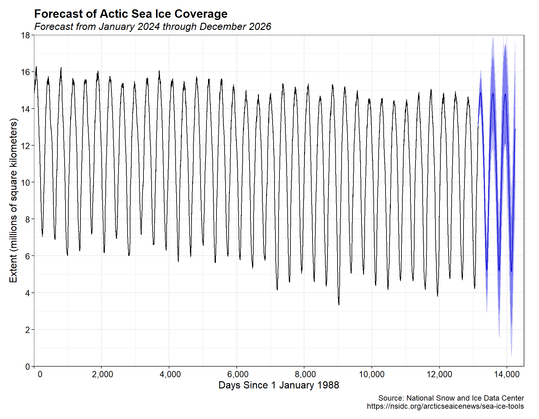
A seasonal auto-regressive integrated moving average (ARIMA) model was fit to the ASIE data. An ARIMA model benefits from low computational requirements and high ease of use for time series analysis. For this model, a regular Fourier cycle of artificial variables was used rather than relying on lagging variables by 365.25 days.
# Pretend no frequency in the call to ts (use later in auto.arima)
seaice_ts1 <- ts(
  seaice_sub$extent,
  frequency = 1,
  start = 0
)

# Use yearly frequency
seaice_ts365 <- ts(
  seaice_sub$extent,
  frequency = 365.25,
  start = 1988
)

# Create K = 5 Fourier terms to model annual seasonality
z <- fourier(seaice_ts365, K = 5)
zf <- fourier(seaice_ts365, K = 5, h = 3*365)

# Fit the model
seaice_model <- auto.arima(seaice_ts1, xreg = z)

# Check residuals
checkresiduals(seaice_model)
##
## 	Ljung-Box test
##
## data:  Residuals from Regression with ARIMA(3,1,3) errors
## Q* = 19.625, df = 4, p-value = 0.0005922
##
## Model df: 6.   Total lags used: 10
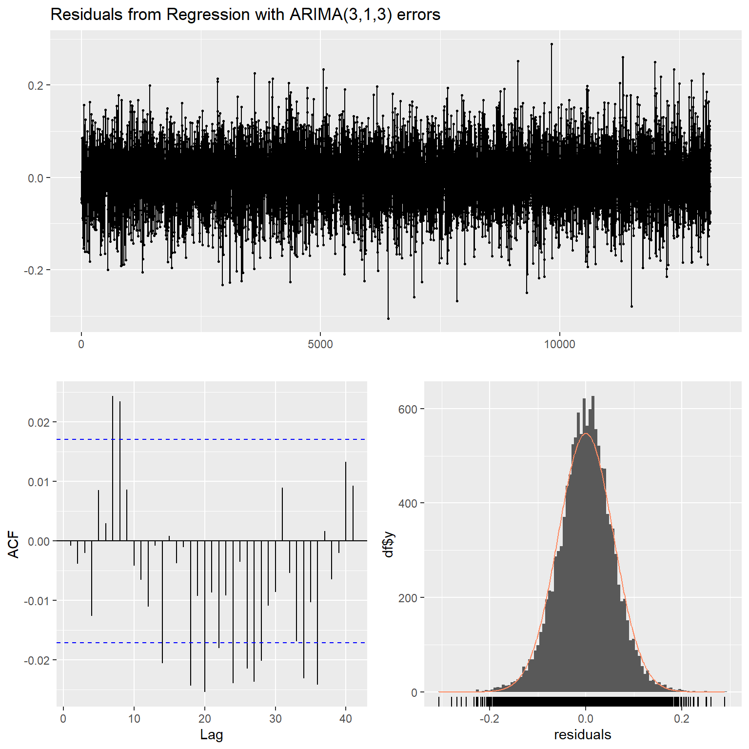
The residuals of the model are not independently distributed but appear to be correlated. Perhaps the model could be improved but this is an exploratory excercise. A plot of the model and a 3-year forecast (January 2024 through December 2026) is shown below. The model predicts a nearly ice-free summer in 2026.
# Forecast using the model
seaice_fc <- forecast(seaice_model, 3*365, xreg = zf)

# Plot results
autoplot(seaice_fc) +
  scale_x_continuous(limits = c(0, 14500),
                     breaks = seq(0, 14000, by = 2000),
                     expand = c(0, 0),
                     labels = function(x) format(x, big.mark = ",",
                                                 scientific = FALSE)) +
  scale_y_continuous(limits = c(0, 18),
                     breaks = seq(0, 18, by = 2),
                     expand = c(0, 0)) +
  labs(title = 'Forecast of Actic Sea Ice Coverage',
       subtitle = 'Forecast from January 2024 through December 2026',
       caption = cap,
       x = 'Days Since 1 January 1988',
       y = 'Extent (millions of square kilometers)') +
  theme_bw() +
  my_theme
Arctic Sea Ice Maps
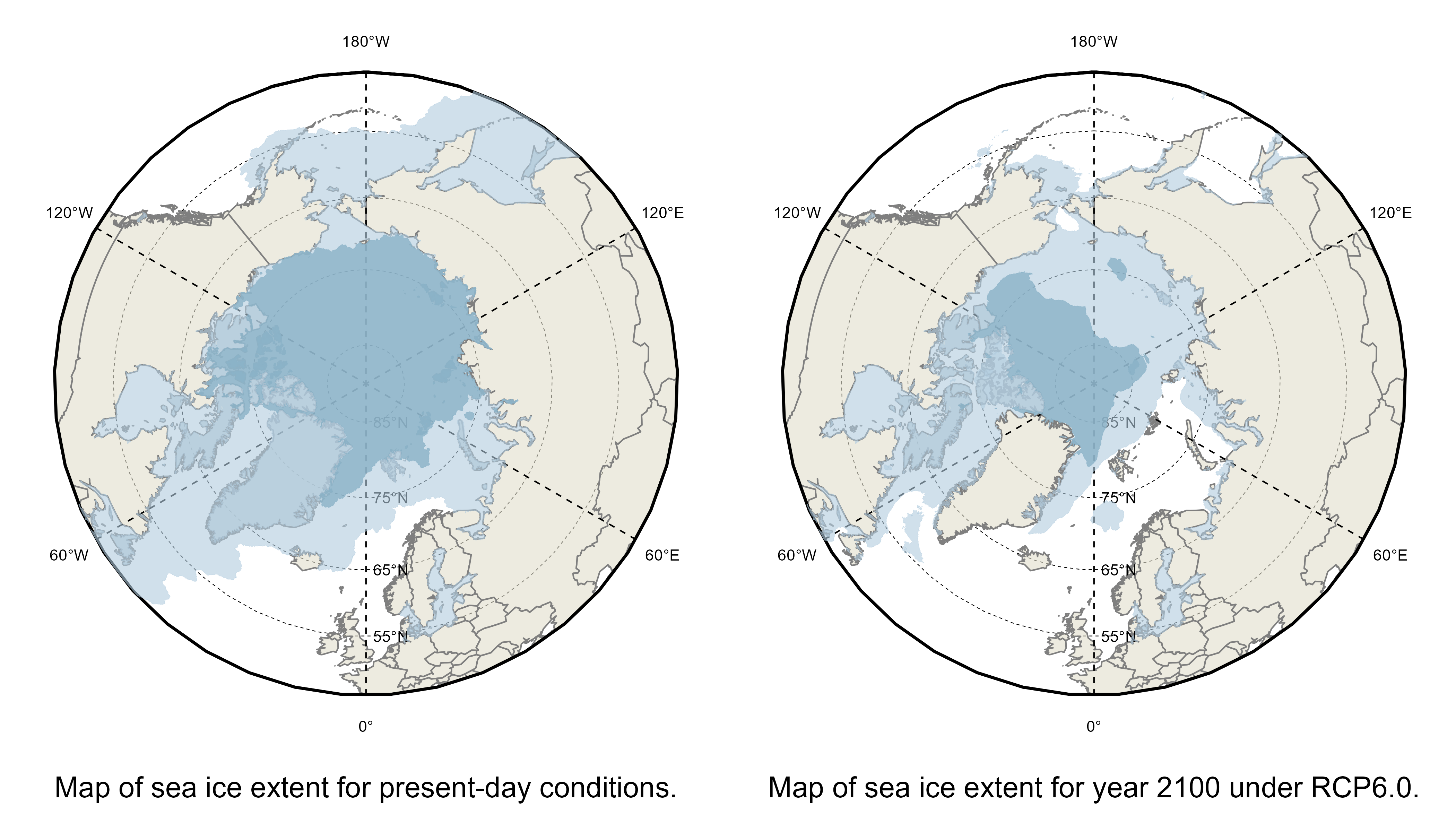
The Arctic is an ocean basin surrounded by continents and mountainous land masses, which limits the expansion of sea ice. In contrast, the Antarctic is a continent surrounded by a vast ocean, allowing sea ice to expand more freely. A map of the Arctic sea ice can be generated using the R package sdmpredictors and information extracted from Bio-ORACLE, an open source dataset of GIS layers that provides geophysical, biotic and environmental data for surface and benthic marine realms. The sdmpredictors package facilitates data extraction from Bio-ORACLE for bioclimatic modelling.
A map of sea ice presence in the Northern Hemisphere around the North Pole for present conditions (defined as the long-term average between 2000 and 2014) is shown below. For comparison a map of sea ice presence in 2100 based on RCP6.0 is also shown. The RCP (Representative Concentration Pathway) number is related to the strength of human influences on the climate at the end of the 21st century where larger numbers are indicative of higher greenhouse gas concentrations. The RCP6.0 scenario uses a medium-high greenhouse gas emission rate (Masui et al. 2011).
# Load libraries
library(sdmpredictors)
library(gridExtra)
library(raster)
library(sf)
library(stars)

# Define extent of map
cExtent <- c(-180, 180, 45, 90)

# Load sea ice thickness raster data
iceMin <- load_layers('BO21_icethickltmin_ss')
iceMax <- load_layers('BO21_icethickltmax_ss')

# Transform sea ice thickness into binomial surface depicting
# presence/absence of sea ice
iceMin[iceMin > 0] <- 1
iceMin[iceMin == 0] <- NA
iceMax[iceMax > 0] <- 1
iceMax[iceMax == 0] <- NA

# Transform sea ice data raster to polygon data
iceMin <- as_Spatial(
  st_as_sf(st_as_stars(iceMin),
  as_points = FALSE, merge = TRUE)
)
iceMax <- as_Spatial(
  st_as_sf(st_as_stars(iceMax),
  as_points = FALSE, merge = TRUE)
)

# Crop ice data to the final exent
iceMin <- crop(buffer(iceMin, width = 0), cExtent)
iceMax <- crop(buffer(iceMax, width = 0), cExtent)

# Load landmasses
data('wrld_simpl', package = 'maptools')
wm <- crop(wrld_simpl, extent(-180, 180, 45, 90))

# Create polar map
x_lines <- seq(-120, 180, by = 60)

# Create basemap
cap <- 'Source: Bio-ORACLE Marine data layers for ecological modeling'
basemap <- ggplot() +
  geom_polygon(data = wm, aes(x = long, y = lat, group = group),
               fill = '#E1DDCB', color = 'grey50', alpha = 0.6) +
  coord_map('ortho', orientation = c(90, 0, 0)) +
  scale_y_continuous(breaks = seq(45, 90, by = 10), labels = NULL) +
  scale_x_continuous(breaks = NULL) +
  labs(caption = cap,
       x = NULL,
       y = NULL) +
  geom_text(aes(x = 0, y = seq(55, 85, by = 10), hjust = -0.2,
            label = paste0(seq(55, 85, by = 10), '°N'))) +
  geom_text(aes(x = x_lines, y = 39,
            label = c('120°W', '60°W', '0°',
                      '60°E', '120°E', '180°W'))) +
  geom_hline(aes(yintercept = 45), size = 1)  +
  geom_segment(aes(y = 45, yend = 90, x = x_lines, xend = x_lines),
               linetype = 'dashed') +
  theme(plot.caption = element_text(size = 12, hjust = 0.5),
        panel.background = element_blank(),
        panel.grid.major = element_line(size = 0.25, linetype = 'dashed',
                             color = 'black'),
        axis.ticks = element_blank())

# Add current ice layers to basemap
iceMapPresent <- basemap +
  geom_polygon(data = iceMax, aes(x = long, y = lat, group = group),
               fill = alpha('#B0CCDE', 0.6), color = NA) +
  geom_path(data = iceMax, aes(x = long, y = lat, group = group),
            color = alpha('#B0CCDE', 0.6), linewidth = 0.1) +
  geom_polygon(data = iceMin, aes( x = long, y = lat, group = group),
               fill = alpha('#89B2C7', 0.8), color = NA) +
  geom_path(data = iceMin, aes(x = long, y = lat, group = group),
            color = alpha('#89B2C7', 0.8), linewidth = 0.1) +
  labs(caption = '\nMap of sea ice extent for present-day conditions.')
iceMapPresent
Generate a projection of sea ice extent for the future (year 2100), under the Representative Concentration Scenario 6.0.
# Load sea ice thickness raster data
iceMin <- load_layers("BO21_RCP60_2100_icethickltmin_ss")
iceMax <- load_layers("BO21_RCP60_2100_icethickltmax_ss")

# Transform sea ice thickness into binomial surface depicting
# presence/absence of sea ice
iceMin[iceMin > 0] <- 1
iceMin[iceMin == 0] <- NA
iceMax[iceMax > 0] <- 1
iceMax[iceMax == 0] <- NA

# Transform sea ice data raster to polygon data
iceMin <- as_Spatial(
  st_as_sf(st_as_stars(iceMin),
  as_points = FALSE, merge = TRUE)
)
iceMax <- as_Spatial(
  st_as_sf(st_as_stars(iceMax),
  as_points = FALSE, merge = TRUE)
)

# Crop ice data to the final exent
iceMin <- crop(buffer(iceMin, width = 0), cExtent)
iceMax <- crop(buffer(iceMax, width = 0), cExtent)

# Add future ice layers to basemap
iceMapFuture <- basemap +
  geom_polygon(data = iceMax, aes(x = long, y = lat, group = group),
               fill = alpha('#B0CCDE', 0.6), color = NA) +
  geom_path(data = iceMax, aes(x = long, y = lat, group = group),
            color = alpha('#B0CCDE', 0.6), linewidth = 0.1) +
  geom_polygon(data = iceMin, aes( x = long, y = lat, group = group),
               fill = alpha('#89B2C7', 0.8), color = NA) +
  geom_path(data = iceMin, aes(x = long, y = lat, group = group),
            color = alpha('#89B2C7', 0.8), linewidth = 0.1) +
  labs(caption = '\nMap of sea ice extent for the year 2100 under RCP6.0.')
Conclusions
Passive-microwave instrumentation on satellites has allowed for the monitoring of Arctic sea ice coverage since the late 1970s, showing a long-term downward trend due to both natural variability and climate change. Studies indicate that approximately half of the decline is caused by natural variability, while the other half is directly linked to climate change (NSIDC 2024). The rate of decline in Arctic sea ice has varied over the past 43 years, with some periods showing faster rates of loss than others. A NSIDC scientist analyzed the long-term trend of Arctic sea ice extent from 1979 to 2021, dividing it into three periods (NSIDC 2024). A downward trend was noted in the early period, the strongest downward trend in the middle period, and a near-zero trend in the late period. It is surmised that natural variability and the resilience of surviving ice in the north may have contributed to the different trend rates.
Sea ice in polar regions is a key factor in climate change, serving as both an indicator and driver with significant societal and ecological implications. It is essential for atmospheric models and serves as a standard for assessing coupled climate models. Sea ice is highly mobile, and although satellite data has indicated a decline in Arctic sea ice since the late 1970s, a decrease in extent does not necessarily imply a corresponding decrease in ice volume. There also exists a contrast between the observable impacts of Arctic changes within the region itself and the uncertainties surrounding the influence of sea ice and Arctic change on areas beyond the Arctic. While the effects of these changes are evident within the Arctic, their repercussions on regions outside the Arctic are not clearly understood or predictable. The interconnected nature of the global climate system complicates the ability to accurately forecast how shifts in Arctic sea ice and environmental conditions will impact other parts of the world. The complexity of these interactions and the presence of various feedback mechanisms make it challenging to determine the exact consequences of Arctic changes on a global scale. This uncertainty underscores the need for further research and understanding of the broader implications of Arctic transformations on the Earth’s climate system.
References
Cleveland, R.B., W.S. Cleveland, J.E. McRae, and I. Terpenning. 1990. STL: A seasonal-trend decomposition procedure based on loess. Journel of Official Statistics 6, 3-73.
Cohen, J., J.A. Screen, J.C. Furtado, M. Barlow, D. Whittleston, D. Coumou, J. Francis, K. Dethloff, D. Entekhabi, J. Overland, and J. Jone. 2014. Recent Arctic amplification and extreme mid-latitude weather. Nat. Geosci. 7, 627-637.
Gregory, J.M., P.A. Stott, D.J. Cresswell, N.A. Rayner, C. Gordon, and D.M.H. Sexton. 2002. Recent and future changes in Arctic sea ice simulated by the HadCM3 AOGCM. Geophys. Res. Lett. 29, 2175.
Huntington, H.P., P.A. Loring, G. Gannon, S.F. Gearheard, S.C. Gerlach, and L.C. Hamilton. 2017. Staying in place during times of change in Arctic Alaska: The implications of attachment, alternatives, and buffering. Reg. Environ. Chang. 17, 897-906.
Kendall, M.G. 1975. Rank Correlation Techniques, 4th ed. Charles Griffen. London.
Laidre, K.L., H. Stern, K.M. Kovacs, L. Lowry, S.E. Moore, E.V. Regehr, S.H. Ferguson, O. Wiig, P. Boveng, R.P. Angliss, E.W Born, D. Litovka, L. Quakenbush, C. Lydersen, D. Vongraven, and F. Ugarte. 2020. Arctic marine mammal population status, sea ice habitat loss, and conservation recommendations for the 21st century. Conserv. Biol. 34, 630-643.
Mann, H.B. 1945. Nonparametric Tests Against Trend. Econometrica, 13, 245-259.
Masui T., K. Matsumoto, Y. Hijioka, T. Kinoshita, T. Nozawa, S. Ishiwatari, E. Kato, P.R. Shukla, Y. Yamagata, and M. Kainuma. 2011. An emission pathway for stabilization at 6 \(Wm^{-2}\) radiative forcing. Clim. Change 109, 59-76.
Meier, W.N., G. Peng, D.J. Scott, M. Savoie, M. 2014. Verification of a new passive microwave sea ice concentration climate data record. Polar Res. 33, 1-22.
Min, S.K., X. Zhang, F.W. Zwiers, and T. Agnew. 2008. Human influence on Arctic sea ice detectable from early 1990s onwards. Geophys. Res. Lett. 35, L21701.
National Snow and Ice Data Center (NSIDC). 2024. Climate change or variability: What rules Arctic sea ice? https://nsidc.org/learn/ask-scientist/climate-change-or-variability-what-rules-arctic-sea-ice. Accessed February 19.
Notz, D. and J. Marotzke. 2012. Observations reveal external driver for Arctic sea-ice retreat. Geophys. Res. Lett. 39, L08502.
Pistone, K., I. Eisenman, and V. Ramanathan. 2019. Radiative Heating of an Ice-Free Arctic Ocean. Geophys. Res. Lett. 46, 7474-7480.
Rantanen, M., A.Y. Karpechko, A. Lipponen, K. Nordling, O. Hyvarinen, K. Ruosteenoja, T. Vihma, and A. Laaksonen. 2022. The Arctic has warmed nearly four times faster than the globe since 1979. Communications Earth & Environment, 3, 1-10.
Screen, J.A. and I. Simmonds, I. 2010. The central role of diminishing sea ice in recent Arctic temperature amplification. Nature 464, 1334-1337.
Sen, P.K. 1968. Estimates of regression coefficient based on kendall’s tau. JASA 63, 1379-1389.
Theil, H. 1950. A rank invariant method of linear and polynomial regression analysis, i, II, III. Proceedings of the Koninklijke Nederlandse Akademie Wetenschappen, Series A - Mathematical Sciences 53, 386-392, 521-525, 1397-1412.
Timmermans, M.L. and J. Marshall. 2020. Understanding Arctic ocean circulation: a review of ocean dynamics in a changing climate. Journal of Geophysical Research: Oceans 125, 1-35.
Vinnikov, K.Y., A. Robock, R.J. Stouffer, J.E. Walsh, C.L. Parkinson, D.J. Cavalieri, J.F. Mitchell, D. Garrett, and V.F. Zakharov. 1999. Global warming and Northern Hemisphere sea ice extent. Science, 286, 1934-1937.
Zhang J, R. Lindsay, A. Schweiger, and M. Steele. 2013. The impact of an intense summer cyclone on 2012 Arctic sea ice retreat. Geophys. Res. Lett. 40.
- Posted on:
- February 22, 2024
- Length:
- 34 minute read, 7219 words
- See Also: