Arctic Sea Ice Time Series Analysis
By Charles Holbert
February 28, 2024
Introduction
The rapid decline of Arctic sea ice has significant environmental impacts, affecting marine ecosystems, wildlife, and indigenous communities. Sea ice plays a vital role in regulating heat transfer between the atmosphere and ocean. Anthropogenic factors play a significant role in this decline, with models highlighting the influence of human activities, such as rising CO2 levels. Addressing these changes and their interconnectedness with the polar climate system is crucial, given the Arctic’s accelerated warming compared to the global average, emphasizing the need for ongoing research and action to reduce further impacts.
In this blog post, time-series analysis of Arctic sea ice extent (ASIE) is performed using the modeltime library within the R environment for statistical computing and visualization.
Libraries
The modeltime library enables time-series analysis and forecasting within R using the tidymodels ecosystem. tidymodels is a collection of packages for modeling and machine learning using tidyverse principles.
# Load libraries
library(lubridate)
library(tidymodels)
library(modeltime)
library(timetk)
library(tidyverse)
Data
Scientists use sea ice extent to measure the amount of sea ice at the poles, defined as the total area of ocean with at least 15% ice concentration. Time-series analysis will be performed using ASIE, in millions of square kilometers, for the Northern hemisphere from 26 October 1978 through 14 February 2024. Data on sea ice extent are available from the National Snow and Ice Data Center (NSIDC) at the University of Colorado.
# Load data
dat <- read_csv('data/SeaIce_Daily_Extent_G02135_v3.0.csv')
A plot of misisng values in the data is shown velow. This plot was generated using the plot_missing() function from the DataExplorer library.
# Inspect missing data using DataExplorer
DataExplorer::plot_missing(dat)
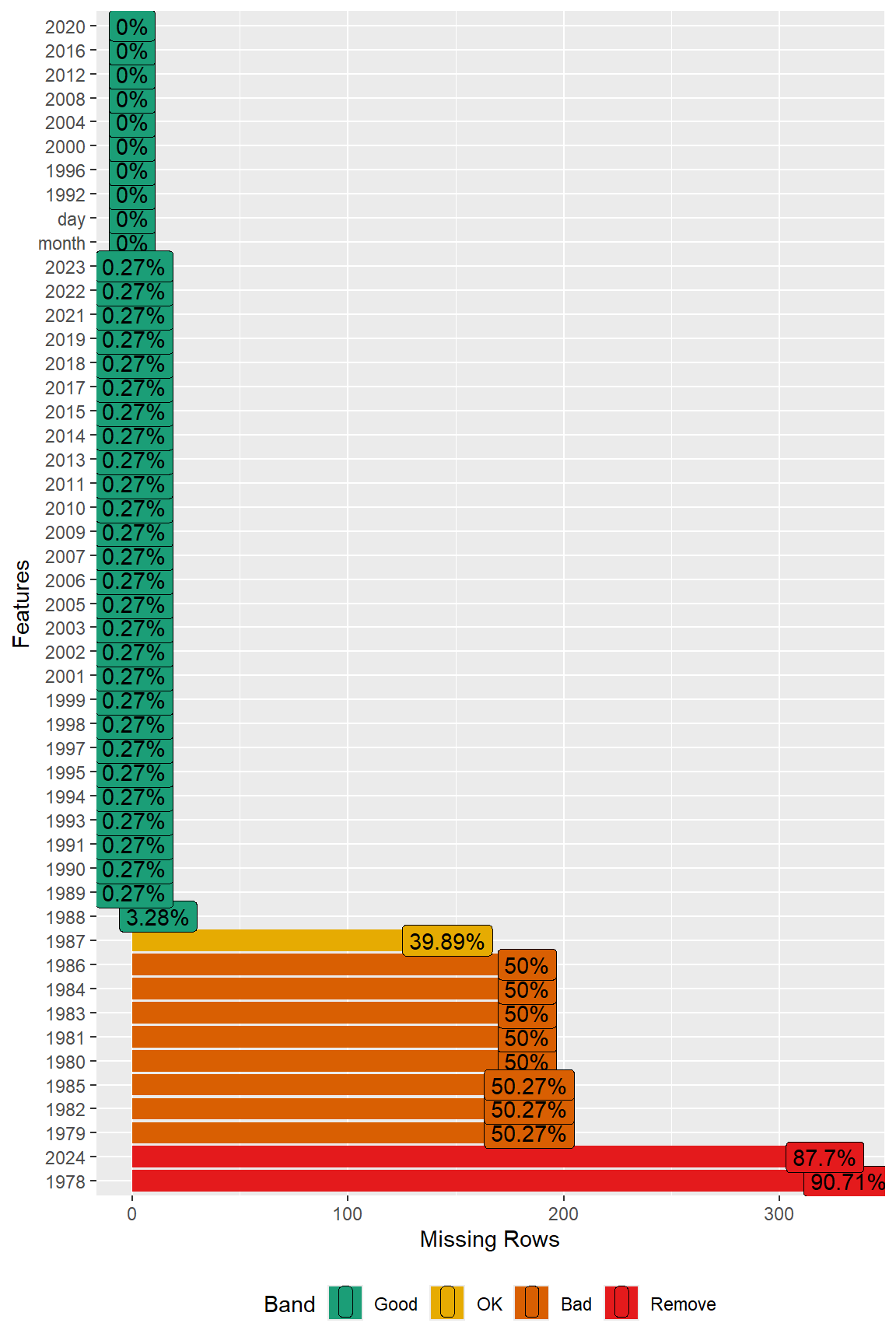
Prior to time-series modeling, those years (1978 through 1987, and 2024) with a significant amount of missing data are removed from the dataset.
# Remove years 1978-1987 and gather data
dat <- dat %>%
  dplyr::select(-as.character(c(seq(1978, 1987, by = 1), 2024))) %>%
  gather(key = 'year', value = 'extent', 3:38) %>%
  mutate(year = as.numeric(year)) %>%
  arrange(year, month, day)
Any remaining missing records are filled in using a “downup” approach that is available in the tidyr library. The “downup” approach fills a missing value first using the previous value or the next value in the time series if there is no previous value.
# Imputate missing values using downup direction
seaice <- dat %>%
  arrange(year, month, day) %>%
  fill(extent, .direction = 'downup') %>%
  mutate(date = as.Date(paste(year, month, day, sep = '-'))) %>%
  filter(!(is.na(date))) %>%  # remove 29 February
  dplyr::select(date, extent) %>%
  set_names(c('date', 'value'))
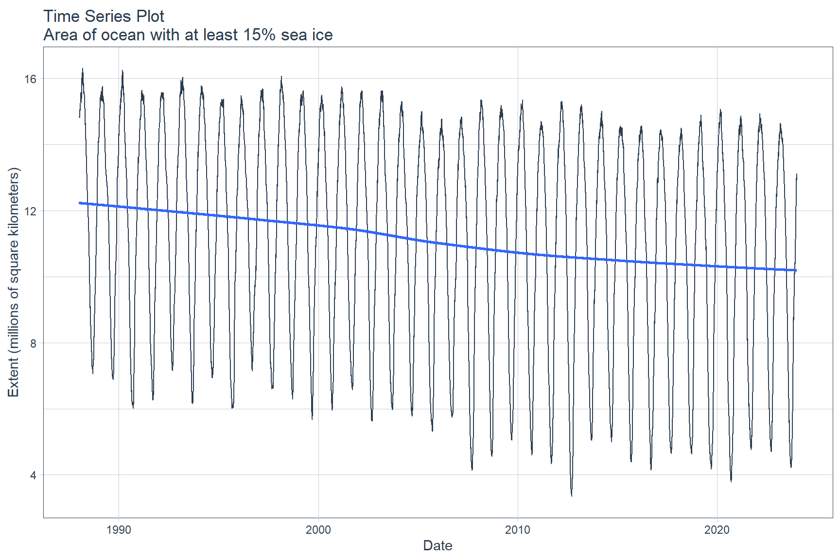
The data can be visualized using the plot_time_series() function from the timetk library.
seaice %>%
  plot_time_series(
    date, value,
   .title = 'Time Series Plot\nArea of ocean with at least 15% sea ice',
    .x_lab = 'Date',
    .y_lab = 'Extent (millions of square kilometers)',
    .interactive = FALSE
  )
Split Data
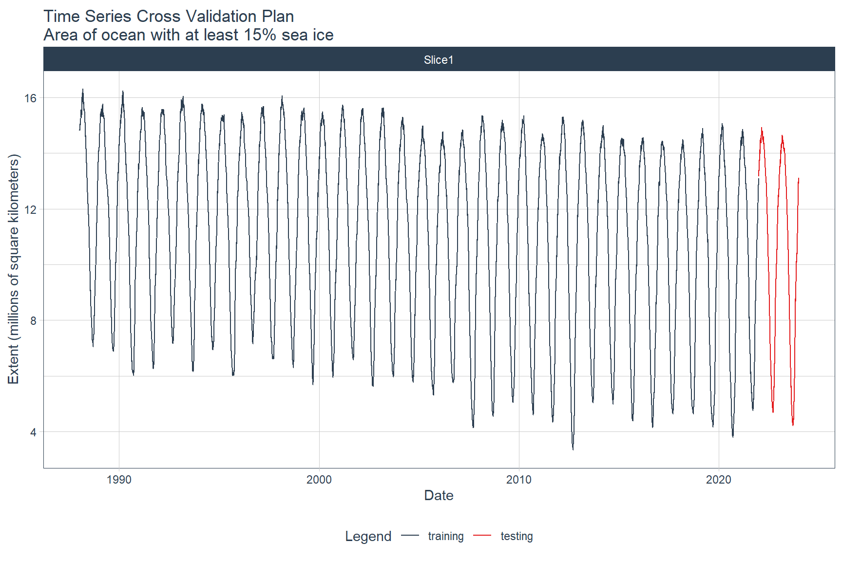
The time series will be split into training and testing sets using the time_series_split() function from the timetk library. The last 24 months of data will be used as the testing dataset. Data prior to the last 24 months will be used as the training dataset.
splits <- seaice %>%
  time_series_split(assess = '24 months', cumulative = TRUE)
The training and testing time series can be visualized by first converting the splits object to a data frame using the tk_time_series_cv_plan() function and then plotting the time series using the plot_time_series_cv_plan() function. Both of these functions are from the timetk library.
splits %>%
  tk_time_series_cv_plan() %>%
  plot_time_series_cv_plan(
    date, value,
   .title = 'Time Series Cross Validation Plan\nArea of ocean with at least 15% sea ice',
    .x_lab = 'Date',
    .y_lab = 'Extent (millions of square kilometers)',
    .interactive = FALSE
  )
Automatic Models
The modeltime library can be used to automatically fit several different types of models, such as Auto ARIMA and Auto ETS from the forecast library and the Prophet algorithm from the prophet library. The process for developing these models is as follows:
-
Model Spec: Use a specification function (e.g., arima_reg() or prophet_reg()) to initialize the algorithm and key parameters
-
Engine: Set an engine using one of the engines available for the Model Spec.
-
Fit Model: Fit the model to the training data
Auto ARIMA
An automatic ARIMA model is fit to the training dataset below. Note that all modeltime models require a date column to be a regressor.
# Fit arima model
model_fit_arima <- arima_reg() %>%
  set_engine('auto_arima') %>%
  fit(value ~ date, training(splits))

model_fit_arima
## parsnip model object
##
## Series: outcome
## ARIMA(3,1,2)
##
## Coefficients:
##         ar1      ar2     ar3      ma1     ma2
##       1.704  -0.7961  0.0878  -1.5347  0.5940
## s.e.  0.086   0.0849  0.0104   0.0860  0.0735
##
## sigma^2 = 0.003552:  log likelihood = 17399.71
## AIC=-34787.43   AICc=-34787.42   BIC=-34742.87
Prophet
Similar to the auto ARIMA model, a Prophet model is fit to the training dataset below. In the model call, seasonality is set to yearly.
# Fit prophet model
model_fit_prophet <- prophet_reg(seasonality_yearly = TRUE) %>%
  set_engine('prophet') %>%
  fit(value ~ date, training(splits))

model_fit_prophet
## parsnip model object
##
## PROPHET Model
## - growth: 'linear'
## - n.changepoints: 25
## - changepoint.range: 0.8
## - yearly.seasonality: 'TRUE'
## - weekly.seasonality: 'auto'
## - daily.seasonality: 'auto'
## - seasonality.mode: 'additive'
## - changepoint.prior.scale: 0.05
## - seasonality.prior.scale: 10
## - holidays.prior.scale: 10
## - logistic_cap: NULL
## - logistic_floor: NULL
## - extra_regressors: 0
Machine Learning Models
Machine learning models are complex and require a structured workflow, often referred to as a pipeline. The general process involves three main steps: (1) create a preprocessing recipe, (2) create model specifications, and (3) use a workflow to combine the model specifications and preprocessing, and fit the model.
Preprocessing
A preprocessing recipe using the recipe() function from the tidymodels library is shown below. This process uses the “date” column to create new time-series features and fourier series for modeling.
recipe_spec <- recipe(value ~ date, training(splits)) %>%
  step_timeseries_signature(date) %>%
  step_rm(contains('am.pm'), contains('hour'), contains('minute'),
          contains('second'), contains('xts')) %>%
  step_fourier(date, period = 365, K = 5) %>%
  step_dummy(all_nominal())

glimpse(recipe_spec %>% prep() %>% juice())
## Rows: 12,418
## Columns: 47
## $ date              <date> 1988-01-01, 1988-01-02, 1988-01-03, 1988-01-04, 198…
## $ value             <dbl> 14.826, 14.826, 14.826, 14.826, 14.826, 14.826, 14.8…
## $ date_index.num    <dbl> 567993600, 568080000, 568166400, 568252800, 56833920…
## $ date_year         <int> 1988, 1988, 1988, 1988, 1988, 1988, 1988, 1988, 1988…
## $ date_year.iso     <int> 1987, 1987, 1987, 1988, 1988, 1988, 1988, 1988, 1988…
## $ date_half         <int> 1, 1, 1, 1, 1, 1, 1, 1, 1, 1, 1, 1, 1, 1, 1, 1, 1, 1…
## $ date_quarter      <int> 1, 1, 1, 1, 1, 1, 1, 1, 1, 1, 1, 1, 1, 1, 1, 1, 1, 1…
## $ date_month        <int> 1, 1, 1, 1, 1, 1, 1, 1, 1, 1, 1, 1, 1, 1, 1, 1, 1, 1…
## $ date_day          <int> 1, 2, 3, 4, 5, 6, 7, 8, 9, 10, 11, 12, 13, 14, 15, 1…
## $ date_wday         <int> 6, 7, 1, 2, 3, 4, 5, 6, 7, 1, 2, 3, 4, 5, 6, 7, 1, 2…
## $ date_mday         <int> 1, 2, 3, 4, 5, 6, 7, 8, 9, 10, 11, 12, 13, 14, 15, 1…
## $ date_qday         <int> 1, 2, 3, 4, 5, 6, 7, 8, 9, 10, 11, 12, 13, 14, 15, 1…
## $ date_yday         <int> 1, 2, 3, 4, 5, 6, 7, 8, 9, 10, 11, 12, 13, 14, 15, 1…
## $ date_mweek        <int> 5, 1, 1, 2, 2, 2, 2, 2, 2, 2, 3, 3, 3, 3, 3, 3, 3, 4…
## $ date_week         <int> 1, 1, 1, 1, 1, 1, 1, 2, 2, 2, 2, 2, 2, 2, 3, 3, 3, 3…
## $ date_week.iso     <int> 53, 53, 53, 1, 1, 1, 1, 1, 1, 1, 2, 2, 2, 2, 2, 2, 2…
## $ date_week2        <int> 1, 1, 1, 1, 1, 1, 1, 0, 0, 0, 0, 0, 0, 0, 1, 1, 1, 1…
## $ date_week3        <int> 1, 1, 1, 1, 1, 1, 1, 2, 2, 2, 2, 2, 2, 2, 0, 0, 0, 0…
## $ date_week4        <int> 1, 1, 1, 1, 1, 1, 1, 2, 2, 2, 2, 2, 2, 2, 3, 3, 3, 3…
## $ date_mday7        <int> 1, 1, 1, 1, 1, 1, 2, 2, 2, 2, 2, 2, 2, 3, 3, 3, 3, 3…
## $ date_sin365_K1    <dbl> 0.06880243, 0.08596480, 0.10310170, 0.12020804, 0.13…
## $ date_cos365_K1    <dbl> 0.9976303, 0.9962982, 0.9946708, 0.9927487, 0.990532…
## $ date_sin365_K2    <dbl> 0.1372788, 0.1712931, 0.2051045, 0.2386728, 0.271958…
## $ date_cos365_K2    <dbl> 0.9905325, 0.9852201, 0.9787401, 0.9711001, 0.962309…
## $ date_sin365_K3    <dbl> 0.2051045, 0.2553533, 0.3049212, 0.3536761, 0.401488…
## $ date_cos365_K3    <dbl> 0.97874008, 0.96684781, 0.95237758, 0.93536795, 0.91…
## $ date_sin365_K4    <dbl> 0.2719582, 0.3375229, 0.4014880, 0.4635503, 0.523415…
## $ date_cos365_K4    <dbl> 0.96230908, 0.94131732, 0.91586429, 0.88607062, 0.85…
## $ date_sin365_K5    <dbl> 0.3375229, 0.4171936, 0.4937756, 0.5667018, 0.635432…
## $ date_cos365_K5    <dbl> 0.94131732, 0.90881764, 0.86958939, 0.82392301, 0.77…
## $ date_month.lbl_01 <dbl> -0.4599331, -0.4599331, -0.4599331, -0.4599331, -0.4…
## $ date_month.lbl_02 <dbl> 0.5018282, 0.5018282, 0.5018282, 0.5018282, 0.501828…
## $ date_month.lbl_03 <dbl> -0.4599331, -0.4599331, -0.4599331, -0.4599331, -0.4…
## $ date_month.lbl_04 <dbl> 0.3687669, 0.3687669, 0.3687669, 0.3687669, 0.368766…
## $ date_month.lbl_05 <dbl> -0.2616083, -0.2616083, -0.2616083, -0.2616083, -0.2…
## $ date_month.lbl_06 <dbl> 0.1641974, 0.1641974, 0.1641974, 0.1641974, 0.164197…
## $ date_month.lbl_07 <dbl> -0.09047913, -0.09047913, -0.09047913, -0.09047913, …
## $ date_month.lbl_08 <dbl> 0.04307668, 0.04307668, 0.04307668, 0.04307668, 0.04…
## $ date_month.lbl_09 <dbl> -0.01721256, -0.01721256, -0.01721256, -0.01721256, …
## $ date_month.lbl_10 <dbl> 0.005456097, 0.005456097, 0.005456097, 0.005456097, …
## $ date_month.lbl_11 <dbl> -0.001190618, -0.001190618, -0.001190618, -0.0011906…
## $ date_wday.lbl_1   <dbl> 3.779645e-01, 5.669467e-01, -5.669467e-01, -3.779645…
## $ date_wday.lbl_2   <dbl> 0.000000e+00, 5.455447e-01, 5.455447e-01, 9.690821e-…
## $ date_wday.lbl_3   <dbl> -4.082483e-01, 4.082483e-01, -4.082483e-01, 4.082483…
## $ date_wday.lbl_4   <dbl> -0.5640761, 0.2417469, 0.2417469, -0.5640761, 0.0805…
## $ date_wday.lbl_5   <dbl> -4.364358e-01, 1.091089e-01, -1.091089e-01, 4.364358…
## $ date_wday.lbl_6   <dbl> -0.19738551, 0.03289758, 0.03289758, -0.19738551, 0.…
The machine learning pipelines for each of the machine learning models are developed below.
Elastic Net
An Elastic Net model for the ASIE training data is created below using linear_reg() and set_engine(“glmnet”) for the model specifications. The glmnet library provides procedures for fitting lasso and elastic-net regularization models for regression, logistic, and multinomial regression.
# Elastic Net model specifications
model_spec_glmnet <- linear_reg(penalty = 0.01, mixture = 0.5) %>%
  set_engine('glmnet')

# Elastic Net workflow
workflow_fit_glmnet <- workflow() %>%
  add_model(model_spec_glmnet) %>%
  add_recipe(recipe_spec %>% step_rm(date)) %>%
  fit(training(splits))
Random Forest
Similar to the Elastic Net model, a Random Forest model for the ASIE training data is created below.
# Random Forest model specifications
model_spec_rf <- rand_forest(trees = 500, min_n = 50) %>%
  set_engine('randomForest') %>%
  set_mode('regression')

# Random Forest workflow
workflow_fit_rf <- workflow() %>%
  add_model(model_spec_rf) %>%
  add_recipe(recipe_spec %>% step_rm(date)) %>%
  fit(training(splits))
Prophet Boost
The modeltime library includes several hybrid models (e.g. arima_boost() and prophet_boost()) that combine automated algorithms with machine learning. The Prophet Boost algorithm combines Prophet with XGBoost to get the best of both worlds (i.e. Prophet Automation plus Machine Learning). The algorithm works by first modeling the univariate series using Prophet and then regressing the Prophet residuals with the XGBoost model.
A Prophet Boost model for the ASIE training data is created below.
# Prophet Boost model specifications
model_spec_prophet_boost <- prophet_boost(seasonality_yearly = TRUE) %>%
  set_engine('prophet_xgboost')

# Prophet Boost workflow
workflow_fit_prophet_boost <- workflow() %>%
  add_model(model_spec_prophet_boost) %>%
  add_recipe(recipe_spec) %>%
  fit(training(splits))

workflow_fit_prophet_boost
## ══ Workflow [trained] ══════════════════════════════════════════════════════════
## Preprocessor: Recipe
## Model: prophet_boost()
##
## ── Preprocessor ────────────────────────────────────────────────────────────────
## 4 Recipe Steps
##
## • step_timeseries_signature()
## • step_rm()
## • step_fourier()
## • step_dummy()
##
## ── Model ───────────────────────────────────────────────────────────────────────
## PROPHET w/ XGBoost Errors
## ---
## Model 1: PROPHET
##  - growth: 'linear'
##  - n.changepoints: 25
##  - changepoint.range: 0.8
##  - yearly.seasonality: 'TRUE'
##  - weekly.seasonality: 'auto'
##  - daily.seasonality: 'auto'
##  - seasonality.mode: 'additive'
##  - changepoint.prior.scale: 0.05
##  - seasonality.prior.scale: 10
##  - holidays.prior.scale: 10
##  - logistic_cap: NULL
##  - logistic_floor: NULL
##
## ---
## Model 2: XGBoost Errors
##
## xgboost::xgb.train(params = list(eta = 0.3, max_depth = 6, gamma = 0,
##     colsample_bytree = 1, colsample_bynode = 1, min_child_weight = 1,
##     subsample = 1), data = x$data, nrounds = 15, watchlist = x$watchlist,
##     verbose = 0, objective = "reg:squarederror", nthread = 1)
Model Evaluation
The modeltime library provides an efficient framework for model evaluation, selection, and forecasting. The Modeltime Table organizes the models with IDs and creates generic descriptions to help keep track of each model. The modeltime_table() function is used below to create a table containing the ASIE models previoulsy developed.
model_table <- modeltime_table(
  model_fit_arima,
  model_fit_prophet,
  workflow_fit_glmnet,
  workflow_fit_rf,
  workflow_fit_prophet_boost
)

model_table
## # Modeltime Table
## # A tibble: 5 × 3
##   .model_id .model     .model_desc
##       <int> <list>     <chr>
## 1         1 <fit[+]>   ARIMA(3,1,2)
## 2         2 <fit[+]>   PROPHET
## 3         3 <workflow> GLMNET
## 4         4 <workflow> RANDOMFOREST
## 5         5 <workflow> PROPHET W/ XGBOOST ERRORS
The modeltime_calibrate() function is used below to perform model calibration using the out-of-sample data (testing dataset). This function generates two new columns (“.type” and “.calibration_data”). The “.calibration_data” contains the actual values, fitted values, and residuals for the testing dataset.
calibration_table <- model_table %>%
  modeltime_calibrate(testing(splits))

calibration_table
## # Modeltime Table
## # A tibble: 5 × 5
##   .model_id .model     .model_desc               .type .calibration_data
##       <int> <list>     <chr>                     <chr> <list>
## 1         1 <fit[+]>   ARIMA(3,1,2)              Test  <tibble [731 × 4]>
## 2         2 <fit[+]>   PROPHET                   Test  <tibble [731 × 4]>
## 3         3 <workflow> GLMNET                    Test  <tibble [731 × 4]>
## 4         4 <workflow> RANDOMFOREST              Test  <tibble [731 × 4]>
## 5         5 <workflow> PROPHET W/ XGBOOST ERRORS Test  <tibble [731 × 4]>
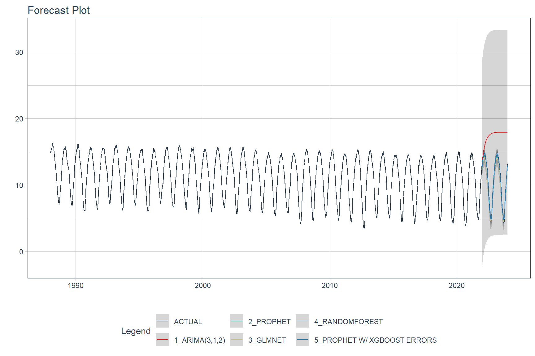
Predictions (forecasts) from the ASIE models applied to the testing data are shown below.
calibration_table %>%
  modeltime_forecast(actual_data = seaice) %>%
  plot_modeltime_forecast(.interactive = FALSE)
A comparions of the testing accuracy for each model is tabulated below.
calibration_table %>%
  modeltime_accuracy() %>%
  table_modeltime_accuracy(.interactive = FALSE)
| Accuracy Table | ||||||||
| .model_id | .model_desc | .type | mae | mape | mase | smape | rmse | rsq |
|---|---|---|---|---|---|---|---|---|
| 1 | ARIMA(3,1,2) | Test | 6.79 | 92.04 | 98.42 | 52.37 | 7.88 | 0.18 |
| 2 | PROPHET | Test | 0.42 | 4.10 | 6.10 | 4.16 | 0.48 | 0.99 |
| 3 | GLMNET | Test | 0.59 | 6.01 | 8.59 | 6.17 | 0.68 | 0.99 |
| 4 | RANDOMFOREST | Test | 0.29 | 3.33 | 4.26 | 3.37 | 0.35 | 0.99 |
| 5 | PROPHET W/ XGBOOST ERRORS | Test | 0.23 | 2.75 | 3.40 | 2.73 | 0.29 | 0.99 |
The model that provides the best fit to the testing data is the Prophet Boost model, a hybrid model that combines Prophet with XGBoost. The worst performing model is the Auto ARIMA model.
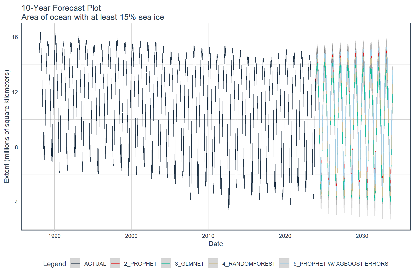
Final Model Predictions
Final model predictions are shown below. Except for the Auto ARIMA model, the models were re-trained on the full ASIE time-series data. The Auto ARIMA model was excluded from the final model predictions because it did not fit the test data very well. The remaining models were used to forecast 10 years into the future, starting in January 2024.
calibration_table %>%
  # Remove ARIMA model with low accuracy
  filter(.model_id != 1) %>%

  # Refit and Forecast Forward
  modeltime_refit(seaice) %>%
  modeltime_forecast(h = "120 months", actual_data = seaice) %>%
  plot_modeltime_forecast(
    .title = '10-Year Forecast Plot\nArea of ocean with at least 15% sea ice',
    .x_lab = 'Date',
    .y_lab = 'Extent (millions of square kilometers)',
    .interactive = FALSE
  )
Conclusions
The modeltime library offers a wide range of features beyond what has been covered in this post. This includes feature engineering, hyperparameter tuning for ARIMA and machine learning models, scalability for handling numerous time series, understanding the strengths and weaknesses of different models, and exploring the potential of implementing Recurrent Neural Networks (RNNs) for time series analysis.
Using the modeltime library, predictions suggest that the Arctic sea will be nearly ice-free in the very near future. This prediction highlights the importance of sea ice in polar regions for climate change and its significant societal and ecological impacts. While the effects of Arctic changes are evident, their impact on areas outside the region remains uncertain due to the complexity of the global climate system. Further research is necessary to understand the broader implications of Arctic alterations on the Earth’s climate system.
- Posted on:
- February 28, 2024
- Length:
- 13 minute read, 2601 words
- See Also: