Introduction

A well-developed sampling design is crucial for scientifically based decision making. It ensures that data collected are representative of the study area and can accurately measure parameter variations, process conditions, or environmental conditions. Representative samples, obtained through random or stratified sampling, play a vital role in minimizing data uncertainty and are necessary for making sound conclusions.

There are two main types of sampling design, namely, statistical (i.e., probabilistic) sampling and judgmental sampling. Statistical sampling involves selecting portions of the material being sampled with an equal chance of selection, known as equiprobability. If certain portions are unavailable, it introduces bias, although the magnitude and nature of the bias cannot be determined. In contrast to statistical sampling, judgmental sampling involves the subjective selection of sampling locations based on expert knowledge or nonrandom criteria. It lacks a basis for quantifying uncertainty in statistical analysis results and cannot be used to generalize results to the larger data population. The objective of judgmental sampling is often an attempt to locate hot spots and involves an authoritative bias.

The post uses the R language for statistical analysis and data visualization to compare differences between simple random sampling and geographically stratified sampling. Simple random sampling is the most fundamental type of statistical or probabilistic sampling design, where the sampling location selection is entirely randomized, with each member of the underlying data population equally likely to be selected as part of the data sample. Stratified sampling involves dividing the target population into distinct units, or strata, and selecting random samples from within each stratum. The sampling variance for stratified sampling is often equal to or better than that obtained through simple random sampling. Generally, simple random sampling is simpler to implement than stratified sampling, but may result in the clustering of samples and large unsampled areas.

Comparison of methods will be based on how well they estimate a global, nonspatial statistic, namely, estimating the population mean. Sampling plans that are effective at estimating the global mean tend to be effective in other areas as well. Different sampling patterns are compared using Monte Carlo simulations on a simulated population. However, it is emphasized that these comparisons do not provide general conclusions about the effectiveness of the patterns for sampling other populations. Nevertheless, this approach contributes to a better understanding of the issues related to spatial sampling.

Simulated Population

The simulated population was generated using a data set and procedures summarized by Plant (2012, p. 128; see Section 5.2.1). The data represent 1996 yield data from an agricultural field measuring 720 meters (m) long by 360 m wide that was planted with wheat. To create an artificial population whose characteristics closely resemble those of a continuously varying population, inverse distance weighted interpolation was conducted using a 5-m x 5-m rectilinear grid, corresponding to a total of 10,368 points.

First, let’s load the main R libraries that will be used for creating the simulated population and for comparing the two sampling methods.

# Load libraries
library(dplyr)
library(rgdal)
library(maptools)
library(gstat)
library(sf)
library(ggplot2)

Let’s load the wheat yield data.

# Load data
dat <- read.csv('data/wheatyield.csv', header = TRUE)

# Make data geospatial object
coordinates(dat) <- c('Easting', 'Northing')
proj4string(dat) <- CRS('+proj=utm +zone=10 +ellps=WGS84')

Let’s create the 5-m by 5-m grid for interpolation.

# Set grid parameters
Left <- 592102.5
Right <- 592817.5
Top <- 4267857.5
Bottom <- 4267502.5
cell.size <- 5

# Create grid 5 meters by 5 meters
grid.xy <- expand.grid(
  x = seq(Left, Right, cell.size),
  y = seq(Top, Bottom, -cell.size)
)
coordinates(grid.xy) <- ~x + y
gridded(grid.xy) = TRUE
proj4string(grid.xy) <- CRS('+proj=utm +zone=10 +ellps=WGS84')

Let’s interpolate the data to the 5-m by 5-m grid using inverse distance weighting.

# Interpolate using IDW
yield.idw <- krige(Yield ~ 1, dat, grid.xy)

## [inverse distance weighted interpolation]

# Add coordinates to IDW results
pop.data <- data.frame(yield.idw@data$var1.pred)
grid.xy <- expand.grid(
  Easting = seq(Left, Right, cell.size),
  Northing = seq(Top, Bottom, -cell.size)
)
coordinates(pop.data) <- grid.xy
names(pop.data) <- 'Yield'
proj4string(pop.data) <- CRS('+proj=utm +zone=10 +ellps=WGS84')

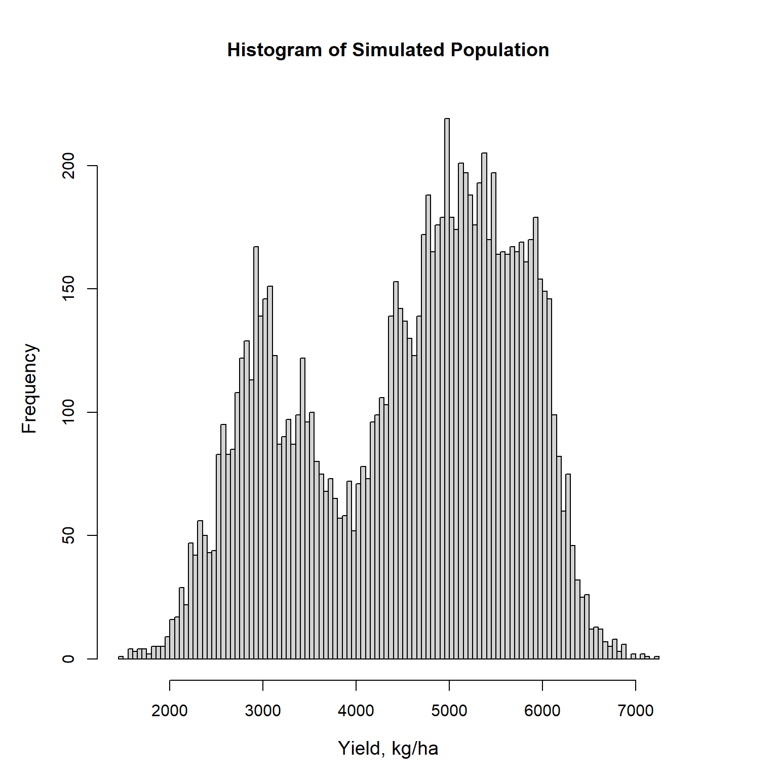
The mean and standard deviation of the simulated population are 4,530 kilograms per hectare (kg/ha) and 1,163 kg/ha, respectively.

# Calculate mean and sd of simulated population
print(pop.mean <- mean(pop.data$Yield), digits = 5)

## [1] 4529.8

print(pop.sd <- sd(pop.data$Yield), digits = 5)

## [1] 1163.3

A histogram of the simulated population is shown below and indicates the population is bimodal. Plant (2012) report that areas with low yield correspond to those areas with high weed levels.

# Create histogram of simulated population
par(mai = c(1, 1, 1, 1))
hist(
  pop.data$Yield, 100, plot = TRUE,
   main = 'Histogram of Simulated Population',
   xlab = 'Yield, kg/ha', font.lab = 1.2, cex.main = 1.2,
   cex.lab = 1.2
)

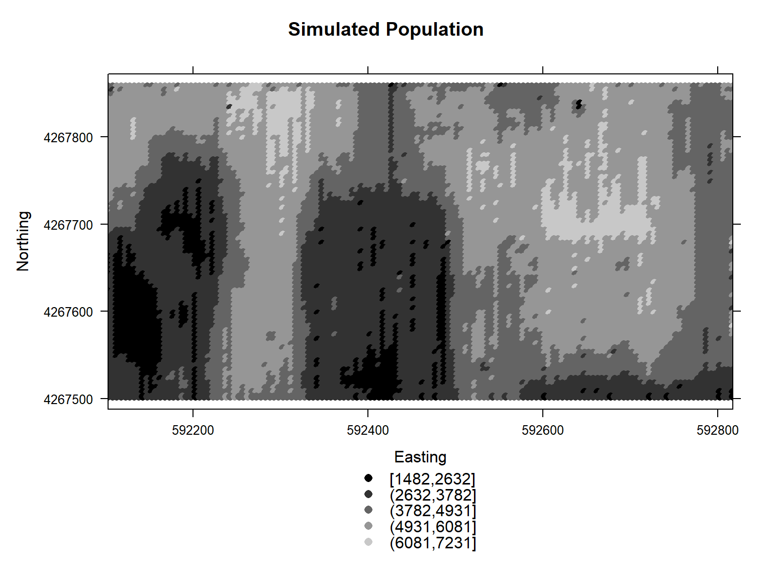
A gray-scale plot of the simulated population is shown below.

# Create grey-scale plot of simulated population
greys <- grey(0:200 / 255)
spplot(
  pop.data, zcol = 'Yield', col.regions = greys,
  xlim = c(Left, Right), scales = list(draw = TRUE),
  xlab = 'Easting', ylab = 'Northing',
  main = 'Simulated Population'
)

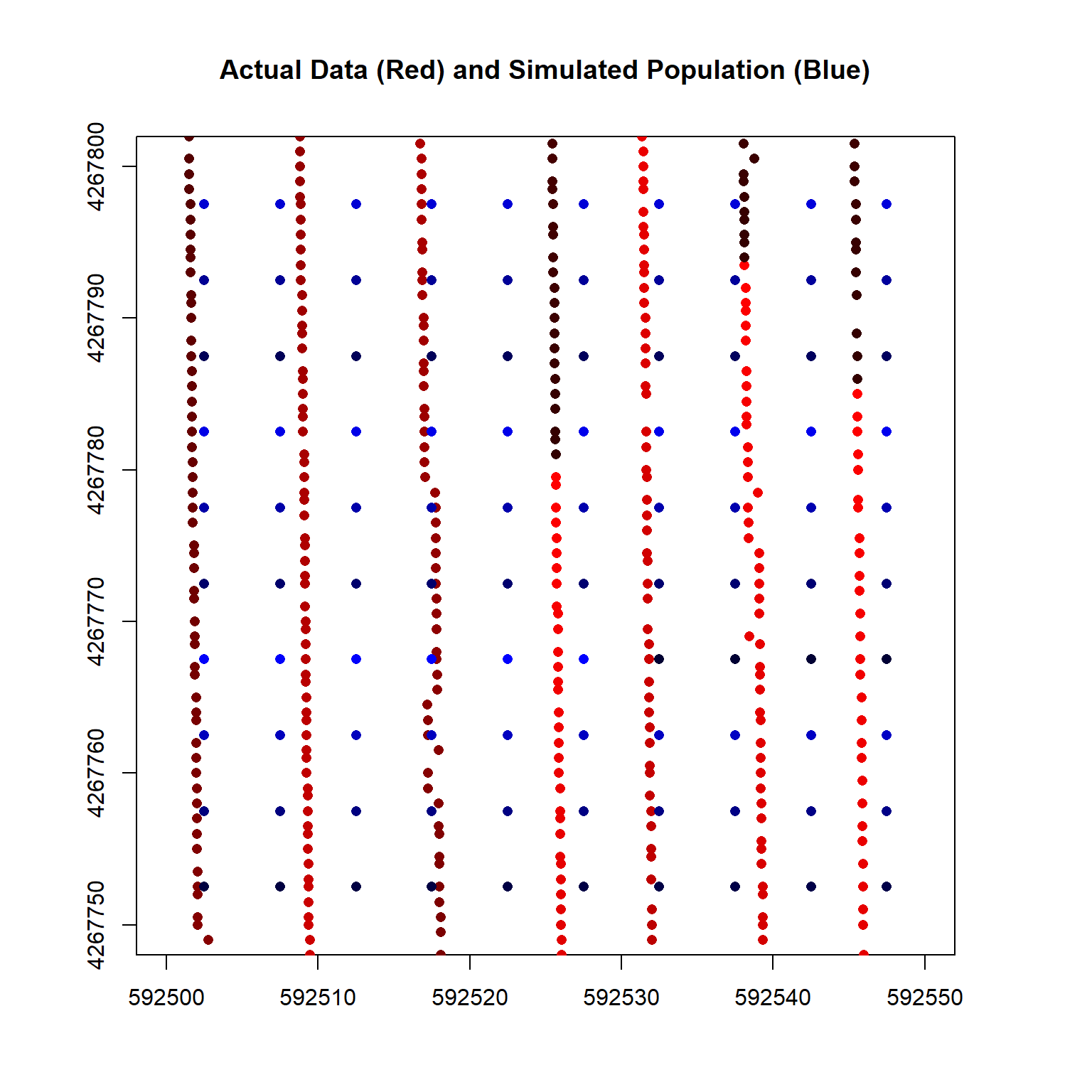
A closeup plot of the simulated population and the actual data is shown below.

# Color version using plot()
reds <- rgb((50:255)/255, green = 0, blue = 0)
par(mai = c(1,1,1,1))
plot(
   dat[,2], axes = TRUE, col = reds, pch = 16,
   xlim = c(592500, 592550), ylim = c(4267750, 4267800),
   main = 'Actual Data (Red) and Simulated Population (Blue)'
)
blues <- rgb((50:255)/255, green = 0, red = 0)
plot(pop.data, add = TRUE, pch = 16, col = blues)

Finally, let’s save the simulated population and corresponding spatial boundary as shapefiles.

# Convert to sf and save to disk
pop.sf <- st_as_sf(pop.data)
st_crs(pop.sf) <- '+proj=utm +zone=10 +ellps=WGS84'
st_write(pop.sf, 'shapes/samplepop.shp')

# Create the sample boundary
W <- bbox(pop.data)[1, 1]
E <- bbox(pop.data)[1, 2]
S <- bbox(pop.data)[2, 1]
N <- bbox(pop.data)[2, 2]
N - S
E - W
N <- N + 2.5
S <- S - 2.5
E <- E + 2.5
W <- W - 2.5
coords.mat <- matrix(c(W,E,E,W,W,N,N,S,S,N), ncol = 2)
coords.lst <- list(coords.mat)
coords.pol = st_sfc(st_polygon(coords.lst))
sampbdry.sf = st_sf(z = 1, coords.pol)
st_crs(sampbdry.sf) <- '+proj=utm +zone=10 +ellps=WGS84'
st_write(sampbdry.sf, 'shapes/samplebdry.shp')

Random vs. Stratified Sampling

Let’s load the shapefiles that were previously created.

# Load shapefile
pop.sf <- st_read('shapes/samplepop.shp')

## Reading layer `samplepop' from data source 
##   `C:\Users\CHolbert\mywebsite\content\blog\random-vs-stratified-sampling\shapes\samplepop.shp' 
##   using driver `ESRI Shapefile'
## Simple feature collection with 10368 features and 1 field
## Geometry type: POINT
## Dimension:     XY
## Bounding box:  xmin: 592102.5 ymin: 4267502 xmax: 592817.5 ymax: 4267858
## Projected CRS: +proj=utm +zone=10 +ellps=WGS84 +units=m +no_defs

pop.data <- as(pop.sf, 'Spatial')
sampbdry.sf <- st_read('shapes/samplebdry.shp')

## Reading layer `samplebdry' from data source 
##   `C:\Users\CHolbert\mywebsite\content\blog\random-vs-stratified-sampling\shapes\samplebdry.shp' 
##   using driver `ESRI Shapefile'
## Simple feature collection with 1 feature and 1 field
## Geometry type: POLYGON
## Dimension:     XY
## Bounding box:  xmin: 592100 ymin: 4267500 xmax: 592820 ymax: 4267860
## Projected CRS: +proj=utm +zone=10 +ellps=WGS84 +units=m +no_defs

sampbdry.sp <- as(sampbdry.sf, 'Spatial')

Random Sampling

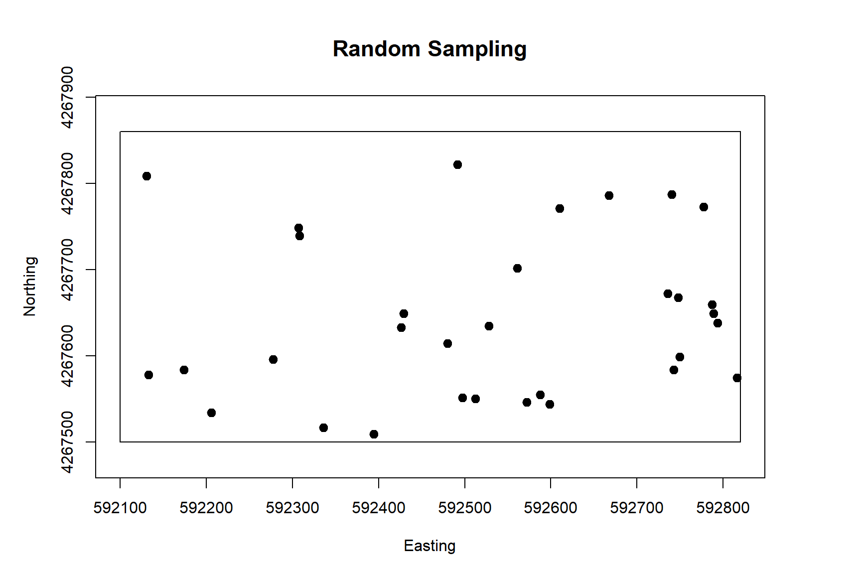
The spsample() function in the sp library can be used for determining sample points within a spatial region. Sample point locations can be determined using regular or random sampling methods within a square area, a grid, a polygon, or along a spatial line. The plot below shows 32 random sample locations within the spatial boundary of our simulated population. Note there a few regions where sample points are clustered together and other regions with no sample points.

# Create simple random sampling using spsample() in sp package
set.seed(123)
spsamp.pts <- spsample(sampbdry.sp, 32, type = 'random')

# Plot the sample points
par(mai = c(1, 1, 1, 1))
plot(sampbdry.sp, axes = TRUE)
plot(spsamp.pts, add = TRUE, pch = 19, cex = 1.2)
title(
  main = 'Random Sampling',
  xlab = 'Easting', ylab = 'Northing',
  cex.main = 1.4, cex.lab = 1, font.lab = 1
)

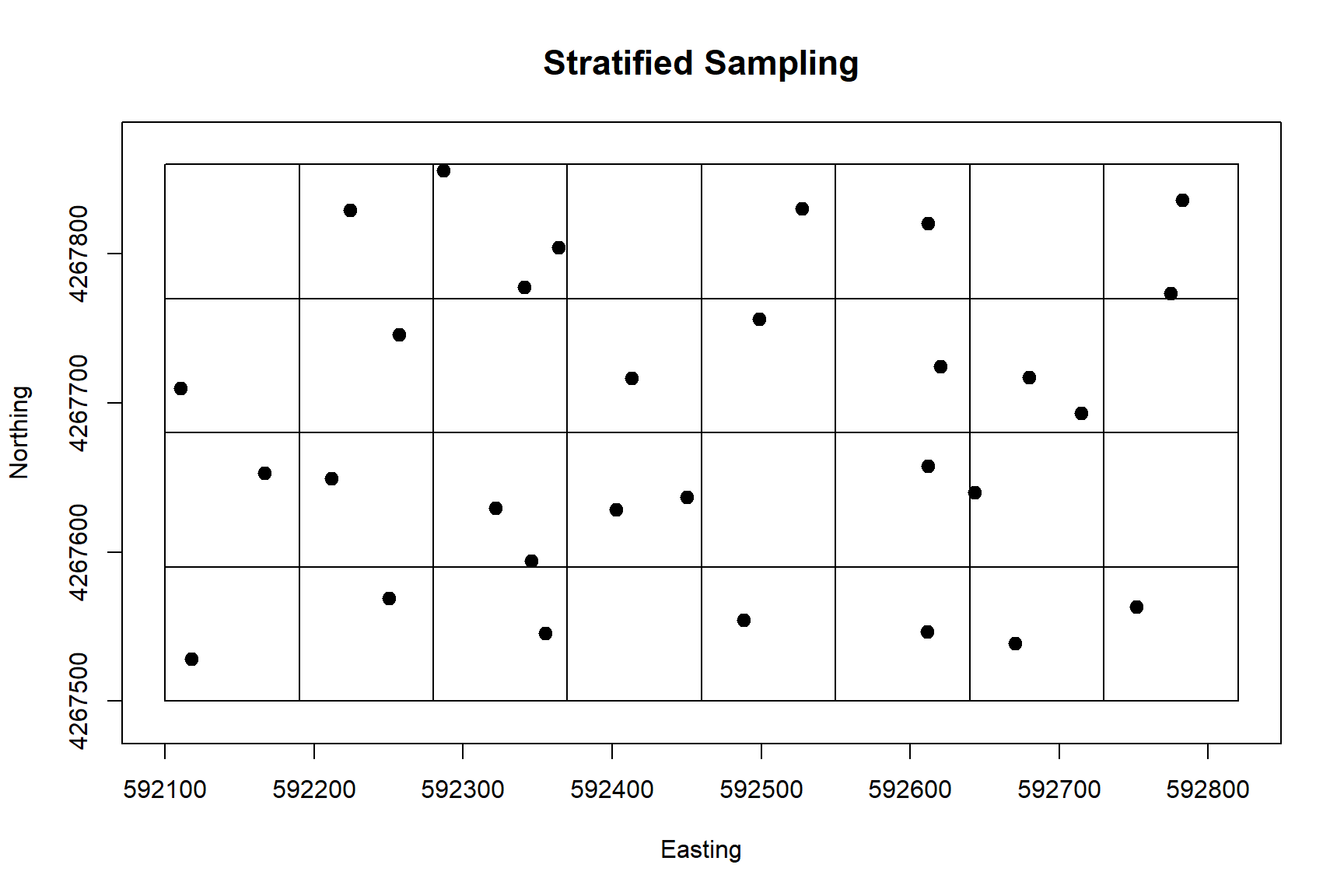
Stratified Sampling

As shown above, a problem with random sampling is that large portions of the site may happen to go unsampled, and some portions may be oversampled. A better spatial distribution of sample point locations can be obtained by stratifying the field geographically and sampling randomly within each stratum. Using this approach, sampling does not miss large geographic regions within the site. Geographic strata of the site can be created using the GridTopology() function in the sp library. For this example, we will assume an 8 x 4 grid, resulting in 32 strata.

# Create sample boundary
W <- bbox(pop.data)[1, 1]
E <- bbox(pop.data)[1, 2]
S <- bbox(pop.data)[2, 1]
N <- bbox(pop.data)[2, 2]
N <- N + 2.5
S <- S - 2.5
E <- E + 2.5
W <- W - 2.5
print(x.size <- (E - W) / 8)

## [1] 90

print(y.size <- (N - S) / 4)

## [1] 90

# Use the GridTopology() function to generate the geographic strata
x.offset <- W + 0.5 * x.size
y.offset <- S + 0.5 * y.size
samp.gt <- GridTopology(
  c(x.offset, y.offset),
  c(x.size, y.size),
  c(8, 4)
)
samp.sp <- as(samp.gt, 'SpatialPolygons')

The spsample() function in the sp library can be used to perform geographically stratified sampling. Stratification is computed internally by the function and is based on sample size. Thus, the stratification does not perfectly match the division of the site that was obtained using the GridTopology() function.

The sample point locations for geographically stratified sampling using the spsample() function are shown in the plot below. Also included in the plot for reference are the 32 strata obtained using the GridTopology() function. It is evident that the sample points are more evenly distributed across the site than those of random sampling

# Create stratified sample of locations
set.seed(123)
samp.size <- 32
plot(samp.sp, axes = TRUE)
title(
  main = 'Stratified Sampling',
  xlab = 'Easting', ylab = 'Northing',
  cex.main = 1.4, font.lab = 1, cex.lab = 1
)
spsamp.pts <- spsample(sampbdry.sp, samp.size, type = 'stratified')
plot(spsamp.pts, pch = 19, cex = 1.2, add = TRUE)

Monte Carlo Simulations

Because the population is limited to 10,368 locations, the random sample points selected by the spsample() function likely will not correspond to actual locations of population members. To address this, let’s develop a function to identify the population member whose location coordinates (x, y) are closest to the random sample point.

# Function to determine population member closest to a sample point
closest.point <- function(sample.pt, grid.data) {
  dist.sq <- (coordinates(grid.data)[,1] - sample.pt[1])^2 +
    (coordinates(grid.data)[,2] - sample.pt[2])^2
  return(which.min(dist.sq))
}

Next, let’s develop two functions for conducting Monte Carlo simulations for both sampling methods. The first function computes the sample mean and the percent error of a random or stratified sample drawn from the population. The second function performs this calculation nsims number of times and returns the mean percent error and the standard deviation of the means.

# Function for random and stratified sampling
sample.design <- function (x) {

  # Create locations of random sample
  if (x[[2]] == 0) samp.type = 'random'
  if (x[[2]] == 1) samp.type = 'stratified'
  
  spsamp.pts <- spsample(sampbdry.sp, x[[1]], type = samp.type)

  # Extract two column array of x and y coords
  sample.coords <- coordinates(spsamp.pts)

  # Apply the function closest.point() to each row of the array sample.coords
  # (i.e., each sample location)
  samp.pts <- apply(sample.coords, 1, closest.point, grid.data = pop.data)

  # Each element of samp.pts is the index of the population value closest to
  # the corresponding location in sample.coords
  data.samp <- pop.data[samp.pts,]
  samp.mean <- mean(data.samp$Yield)
  prct.err <- abs(samp.mean - pop.mean) / pop.mean

  return(c(samp.mean, prct.err))
}

# Function for running Monte Carlo simulations 
simulation <- function (x) {
  dt <- replicate(nsims, sample.design(x))
  list(
    perc.err = mean(dt[2,]),
    sd.mean = sd(dt[1,])
  )
}

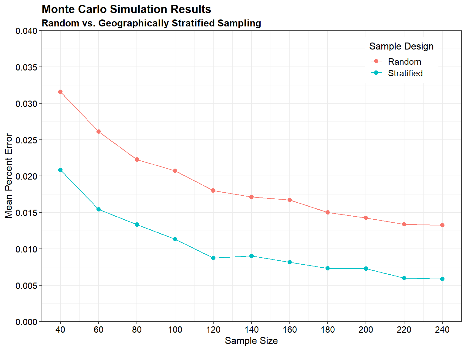
Now, let’s set the number of simulations (nsim) to 1,000 and create a data frame containing our input parameters. Let’s evaluate the mean percent error and the standard deviation of the means for sample sizes ranging from 40 to 240 for both random sampling and geographically stratified sampling.

# Generate data frame of parameters
nsims <- 1000
param <- expand.grid(
  samp.size = seq(40, 240, by = 20),
  samp.type = c(0, 1),
  simreps = nsims
 )

We are now ready to carry out the Monte Carlo simulations.

# Run simulations

###---> Without Parallel Processing

#seed <- 123
#sim.results <- apply(param, 1, simulation)

###---> With Parallel Processing

# Set number of cores
ncores <- 16
if (ncores > parallel::detectCores())
  stop('You requested more cores than are available on the machine.')

# Run simulations
seed <- 123
if (ncores <= 1) {
  if (!is.null(set.seed)) set.seed(seed)
  powers <- apply(param, 1, simulation)
} else {
  cl <- parallel::makeCluster(ncores)
  parallel::clusterExport(
    cl,
    list(
      'nsims', 'pop.data', 'pop.mean', 'sampbdry.sp', 'spsample',
      'coordinates', 'closest.point', 'sample.design'
    )
  )
  if (!is.null(seed)) parallel::clusterSetRNGStream(cl, seed)
  sim.results <- parallel::parApply(cl, param, 1, simulation)
  parallel::stopCluster(cl)
}

# Convert list of lists to dataframe
sim.results.df <- do.call(rbind, lapply(sim.results, as.data.frame))

# Combine output with parameters
param <- bind_cols(param, sim.results.df)

# Change sample type
param <- param %>%
  mutate(samp.type = ifelse(samp.type == 0, 'Random', 'Stratified'))

Let’s compare the mean percent error for random sampling and geographically stratified sampling as a function of sample size.

# Plot results using ggplot2 library
ggplot(data = param, aes(x = samp.size, y = perc.err, color = samp.type)) +
  geom_point(size = 2.2) +
  geom_line(linewidth = 0.4) +
  scale_x_continuous(limits = c(40, 240),
                     breaks = seq(40, 240, 20)) +
  scale_y_continuous(limits = c(0, 0.04),
                     breaks = seq(0, 0.04, 0.005),
                     expand = expansion(mult = c(0, 0))) +
  labs(title = 'Monte Carlo Simulation Results',
       subtitle = 'Random vs. Geographically Stratified Sampling',
       color = 'Sample Design',
       x = 'Sample Size',
       y = 'Mean Percent Error') +
  theme_bw() +
  theme(plot.title = element_text(margin = margin(b = 5), size = 14,
                       hjust = 0, face = 'bold'),
        plot.subtitle = element_text(margin = margin(b = 3), size = 12,
                          hjust = 0, face = 'bold'),
        axis.title = element_text(size = 12, color = 'black'),
        axis.text = element_text(size = 11, color = 'black'),
        legend.title = element_text(size = 12),
        legend.text = element_text(size = 11),
        legend.justification = c(0, 0),
        legend.position = c(0.77, 0.82),
        legend.key.height = unit(1, 'line'))

Conclusions

When interpreting the results of sampling data analysis, it is important to consider whether any biases have been introduced due to imperfections in sample collection. The choice of sampling design is crucial in ensuring that the data collected is representative of the population and can be used for statistical inferences.

Probability-based sampling designs, such as random selection of sampling units, allow for statistical inferences to be made based on the data. Stratified random sampling can improve the spatial distribution of sample point locations compared to simple random sampling. Judgmental sampling designs rely on expert knowledge or professional judgment for the selection of sampling units. While these designs cannot be used to generalize results to the larger population, they can still be useful in certain situations depending on the study objectives, size, scope, and professional judgment available.

All statistical methods to quantify uncertainty assume the use of some form of random sampling. This includes simple random sampling, stratified random sampling, composite sampling, and ranked set sampling. Combining statistical and judgmental sampling can be advantageous, such as including obviously contaminated areas in the data sample regardless of the statistical design.

References

Plant, R.E. 2012. Spatial Analysis in Ecology and Agriculture Uinsg R. CRC Press, Boca Raton, FL.