Introduction

Non-detects in environmental data can complicate analysis and lead to incorrect conclusions if not handled appropriately. Substituting arbitrary values or excluding non-detects can produce poor estimates and bias in statistical measures. When analyzing censored data sets, it is important to employ statistical methods that properly account for non-detects. Most of these methods come from the field of survival analysis, where the primary variable being investigated is length of time. For environmental data, these methods are applied to concentration.

Survival data consists of time-to-event outcomes with distinct start and end times, commonly seen in clinical research, reliability engineering, finance, and event history analysis. These data are often censored or incomplete, meaning that the full information about the event is not known. There are three types of censoring: right censoring, left censoring, and interval censoring. Right censoring occurs when a data point is above a certain value but it is unknown by how much. Left censoring occurs when a data point is below a certain value but it is unknown by how much. Interval censoring occurs when a data point is somewhere within an interval between two values. Left and right censoring are special cases of interval censoring, with the beginning of the interval at zero or the end at infinity, respectively.

Special techniques are used to handle censored data in survival analysis, where specific failure times are coded as actual failures and censored data are coded for the type of censoring and known intervals. The mathematical structure of survival analysis is general enough that it can be used in diverse fields examining various types of data not typically associated with survival/death events or failure analysis.

In this post, survival analysis methods will be used to fit a censored linear regression model to weekly ammonium (NH4) deposition data to test for temporal trend. The analysis will be conducted using the survival package within the R environment for statistical computing and visualization.

Data

Data used for this exercise consist of NH4 concentration in precipitation measured at Olympic National Park, Hoh Ranger Station, weekly or every other week from January 6, 2009 through December 20, 2011. The data were downloaded from the National Atmospheric Deposition Program, National Trends Network (NADP/NTN) and are contained in the EnvStats package. Concentration is given in milligrams-per-liter (mg/L).

# Load libraries
library(dplyr)
library(survival)

# Load data from EnvStats package
data(package = 'EnvStats', 'Olympic.NH4.df')

# Prep data
dat <- Olympic.NH4.df %>%
  mutate(Units = 'mg/L') %>%
  rename(
    NH4.Orig = NH4.Orig.mg.per.L,
    NH4 = NH4.mg.per.L
  ) %>%
  data.frame()

Inspect the data

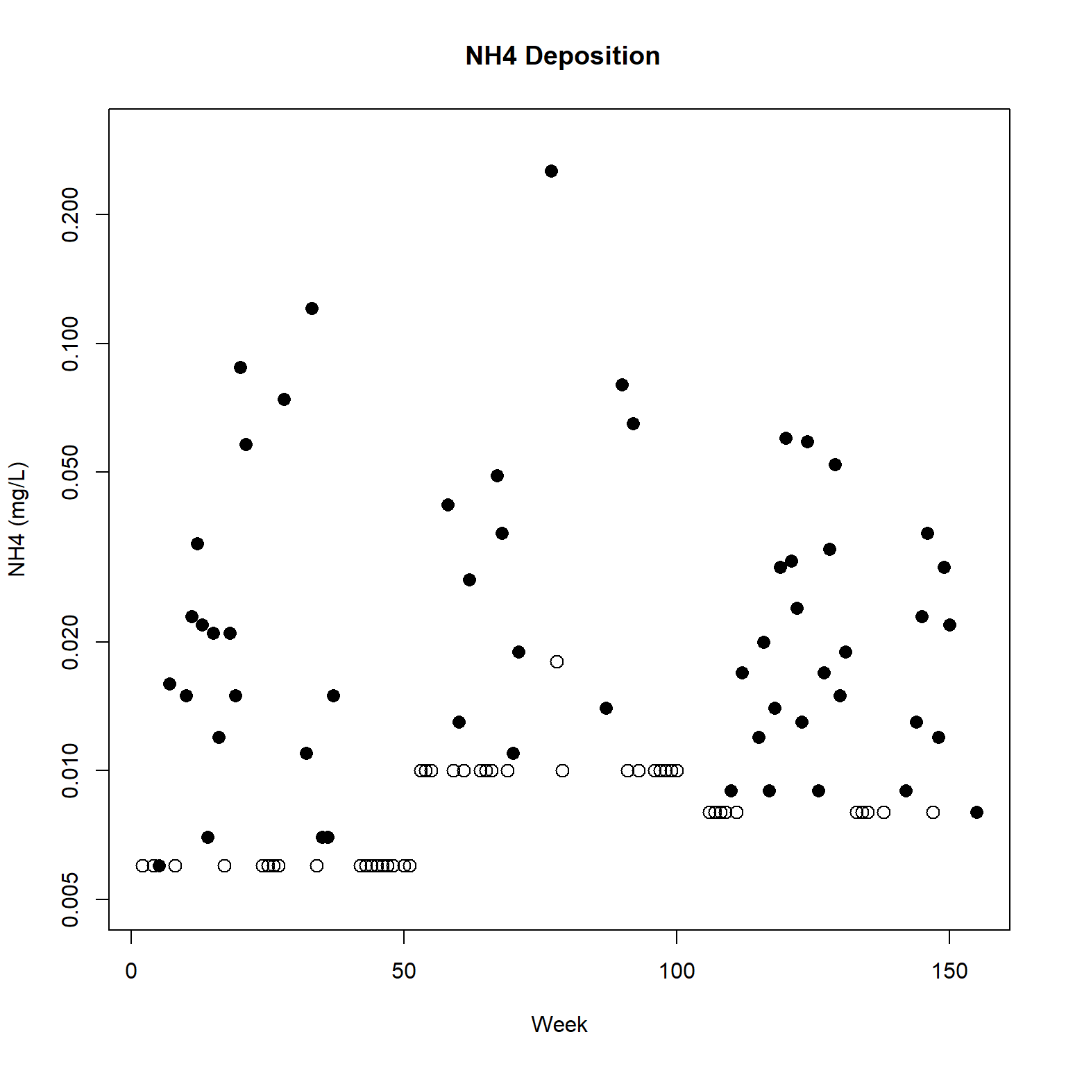
# Plot the data
with(dat,
  plot(
    Week, NH4, type = 'n', log = 'y',
    xlab = 'Week', ylab = 'NH4 (mg/L)',
    main = ' NH4 Deposition', ylim = c(0.005, 0.30)
  )
)
with(dat, points(Week[Censored], NH4[Censored], pch = 1, cex = 1.3))
with(dat, points(Week[!Censored], NH4[!Censored], pch = 16, cex = 1.3))

Survival Object

A key function for the analysis of survival data in R is the Surv() function from the survival package. This is used to specify the type of survival data that we have, namely, right censored, left censored, or interval censored. The Surv() function creates a survival object for use as the response in a model formula. There will be one entry for each observation that is the survival time, which is followed by a “+” if the observation is right censored or “-” if the observation is left censored.

The event variable event in the Surv() function is defined as True = dead (observed value) and False = alive (censored). This is opposite the logical value assigned to non-detects in environmental data. Thus, we will use event = !Censored in the call to the Surv() function. The censoring type is identified as left censoring.

# Create a survival object with left censoring
dat.surv <- with(dat, Surv(time = NH4, event = !Censored, type = 'left'))

Alternatively, the survival object can be created using interval censoring. For internal censoring, each non-detect can be considered as an interval, ranging from negative infinity to the censoring limit. The interval for detected values are simply assigned the measured value. In the Surv() function for interval censored data, the time argument is the starting value for the interval and time2 is the ending time of the interval.

# Create starting value for interval, which is negative infinity for non-detects
dat$NH4.Left = ifelse(dat$Censored == TRUE, -Inf, dat$NH4)

# Create a survival object with interval censoring
dat.surv2 <- with(dat, Surv(time = NH4.Left, time2 = NH4, type = 'interval2'))

Comparing the two objects, we see the numeric values are the same. The only difference between the objects is that dat.surv is classified as left censored while dat.surv2 is classified as interval censored with time1 and time2.

# Compare objects
str(dat.surv)

##  'Surv' num [1:102, 1:2] 0.006- 0.006- 0.006  0.016  0.006- 0.015  0.023  0.034  0.022  0.007  ...
##  - attr(*, "dimnames")=List of 2
##   ..$ : NULL
##   ..$ : chr [1:2] "time" "status"
##  - attr(*, "type")= chr "left"

str(dat.surv2)

##  'Surv' num [1:102, 1:3] 0.006- 0.006- 0.006  0.016  ...
##  - attr(*, "dimnames")=List of 2
##   ..$ : NULL
##   ..$ : chr [1:3] "time1" "time2" "status"
##  - attr(*, "type")= chr "interval"

Censored ECDF

Now that we have a survival object, let’s plot a censored empirical cumulative distribution function (ECDF) for the NH4 data. The survfit() function creates survival curves using the Kaplan-Meier product-limit estimator. The basic output of survfit() gives the number of subjects, the number of events, the median survival time, and its 95% confidence interval. The survminer package can be used to plot the survival curve using the ggplot2 platform. In our case, the survival curve represents the censored ECDF.

# Create survival curve based on Kaplan-Meier estimates
fit.km <- survfit(dat.surv ~ 1, data = dat)
fit.km

## Call: survfit(formula = dat.surv ~ 1, data = dat)
## 
##        n events median 0.95LCL 0.95UCL
## [1,] 102    102  0.009   0.006   0.023

# Plot the survival curve
library(survminer)
ggsurv <- ggsurvplot(
  fit.km, data = dat,
  fun = 'event',
  color = 'gray40', legend = 'none'
)
ggpubr::ggpar(
  ggsurv,
  title = 'Censored ECDF for NH4 Deposition Data',
  xlab = 'Result (mg/L)',
  ylab = 'Cumulative Probability',
  font.legend = list(size = 8, color = 'black')
)

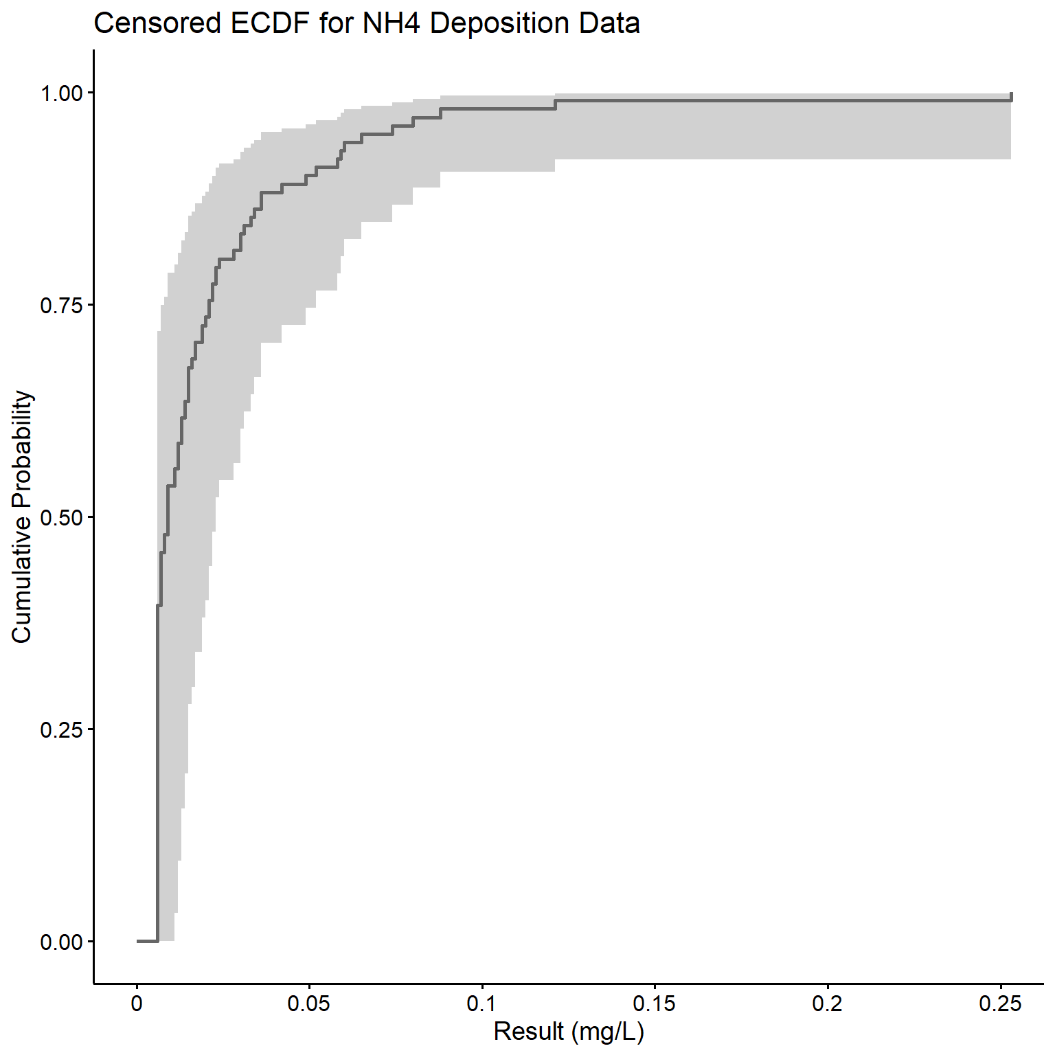
The quantile() function can be used to compute the corresponding concentrations at specific percentiles.

quantile(fit.km, probs = c(0.1, 0.25, 0.5, 0.75, 0.9))

## $quantile
##    10    25    50    75    90 
## 0.006 0.006 0.009 0.021 0.049 
## 
## $lower
##    10    25    50    75    90 
## 0.006 0.006 0.006 0.008 0.022 
## 
## $upper
##    10    25    50    75    90 
## 0.013 0.015 0.023 0.052 0.088

Trend Analysis

Let’s fit a parametric survival regression model assuming a lognormal distribution for NH4, the y variable, and week for the x variable.

dat.trend <- survreg(dat.surv ~ Week, data = dat, dist = 'lognormal')
summary(dat.trend)

## 
## Call:
## survreg(formula = dat.surv ~ Week, data = dat, dist = "lognormal")
##                Value Std. Error      z      p
## (Intercept) -4.99062    0.26791 -18.63 <2e-16
## Week         0.00365    0.00288   1.27  0.204
## Log(scale)   0.21711    0.10369   2.09  0.036
## 
## Scale= 1.24 
## 
## Log Normal distribution
## Loglik(model)= 89   Loglik(intercept only)= 88.2
## 	Chisq= 1.61 on 1 degrees of freedom, p= 0.2 
## Number of Newton-Raphson Iterations: 3 
## n= 102

The p-value for week is 0.2, indicating little evidence of a linear trend over time.

Seasonal Trend Analysis

The plot of the NH4 data suggests the possible presence of seasonality in the data, with low deposition in winter (i.e., around week 0, week 52, week 104). Patterns in deposition over time can be visualized by regressing NH4 on a polynomial spline or a natural-cubic spline representation of week. The survreg() function can fit both using the spline functions bs() for the polynomial basis and ns() for natural-cubic split basis.

First, let’s fit both splines with knots every 26 weeks to capture the annual rise and fall of NH4 deposition. After fitting the splines, let’s inspect a plot of the results.

library(splines)
dat.poly <- survreg(
  dat.surv ~ bs(Week, knots = seq(26, 150, 26)),
  data = dat, dist = 'lognormal'
)

dat.cubic <- survreg(
  dat.surv ~ ns(Week, knots = seq(26, 150, 26)),
  data = dat, dist = 'lognormal'
)

# Plot the data and both regressions
with(dat,
  plot(
    Week, NH4, type = 'n', log = 'y',
    xlab = 'Week', ylab = 'NH4 (mg/L)',
    main = ' NH4 Deposition With Spline Regression',
    ylim = c(0.002, 0.30)
  )
)
with(dat, points(Week[Censored], NH4[Censored], pch = 1, cex = 1.3))
with(dat, points(Week[!Censored], NH4[!Censored], pch = 16, cex = 1.3))

# Add predictions
newx <- seq(5, 155, length.out = 200)
lines(newx, predict(dat.poly, data.frame(Week = newx)), lwd = 2)
lines(newx, predict(dat.cubic, data.frame(Week = newx)), lty = 2, lwd = 2)
legend(
  x = 115, y = 0.3, bty = 'n', 
  legend = c('Polynomial', 'Cubic'), lty = c(1,2), lwd = 2
)

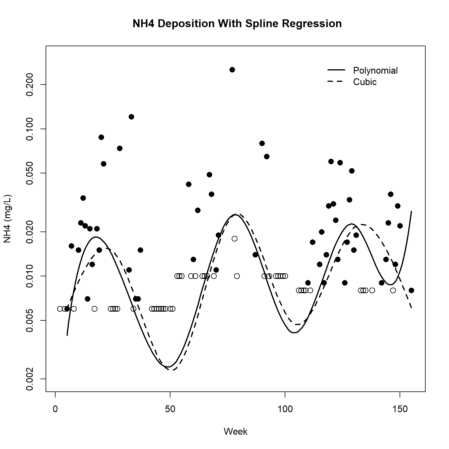
Based on the plot, it appears the data do exhibit seasonality. One approach to model seasonality and trend is to describe the seasonal patterns by a trignometric regression using sine and cosine terms. The term sin(2 x pi x week / 52) represents one year as a full cycle.

dat.trend <- survreg(
  dat.surv ~ I(sin(2*pi*Week/52)) + I(cos(2*pi*Week/52)) + Week,
  data = dat, dist = 'lognormal'
)
summary(dat.trend)

## 
## Call:
## survreg(formula = dat.surv ~ I(sin(2 * pi * Week/52)) + I(cos(2 * 
##     pi * Week/52)) + Week, data = dat, dist = "lognormal")
##                             Value Std. Error      z       p
## (Intercept)              -5.13595    0.26094 -19.68 < 2e-16
## I(sin(2 * pi * Week/52))  0.38307    0.17332   2.21 0.02709
## I(cos(2 * pi * Week/52)) -0.72432    0.19191  -3.77 0.00016
## Week                      0.00495    0.00270   1.83 0.06672
## Log(scale)                0.10916    0.10214   1.07 0.28521
## 
## Scale= 1.12 
## 
## Log Normal distribution
## Loglik(model)= 99   Loglik(intercept only)= 88.2
## 	Chisq= 21.68 on 3 degrees of freedom, p= 7.6e-05 
## Number of Newton-Raphson Iterations: 4 
## n= 102

Evidence for a linear trend, after adjusting for seasonal effects modeled as a sine curve and cosine curve, is weak. The p-value for trend is 0.067, which is suggestive evidence of a trend in the data. The estimated trend is 0.00495 per week (0.26 per year) with a standard error of 0.0027 per week (0.14 per year).