Introduction

A common problem that arises in statistical data analysis is the comparison of two, independent groups of data. Generally, two-sample hypothesis tests are used to compare the means, medians, or other percentiles of the two populations to determine if there is a significant difference between the groups. The goal is to use the estimate of the mean (or other central measure), assess the variation based on sample estimates, and use this information to determine if there is a statistically significant difference in means or central tendency. Typically, for a given N (i.e., total sample size), statistical power is maximized if the sample sizes for each group are equal. With highly unequal group sizes, each additional observation adds little additional resolution.

This simulation study focuses on determining the effect of unequal sample sizes on the statistical power of two-sample hypothesis tests, assuming independent samples with equal variance. Simulations will be conducted using the R language for statistical computing and visualization.

Background

There are several different methods that can be used to determine whether the difference between two groups of data is statistically significant. If the data in each group are normally distributed, a two-sample t-test (see Lehmann and Romano 2005) can be used to compare the means of the two groups. If this assumption is severely violated, the nonparametric Wilcoxon Rank Sum (WRS) test (Wilcoxon 1945), also known as the two-sample Mann-Whitney U test (Mann and Whitney 1947), may be considered instead. This is a nonparametric version of a two-sample t-test and calculates whether the medians of the two distributions are different or similar, assuming observations in each group are identically and independently distributed apart from location. When observations represent very different distributions, the method is a test of dominance between distributions. Another alternative is a two-sample permutation test (see Good 2001). The two-sample permutation test works by enumerating all possible permutations of group assignments, and for each permutation computing the difference between the measures of location for each group. At the end of the test, the actual difference observed between the two groups is compared with the thousands of simulations performed to see how likely or unlikely it would be under the null hypothesis. Permutation tests compute the p-value using computer-intensive methods rather than assuming data follow normal distributions and thus, avoid the normality assumption of the parametric t-test.

Statistical Approach

Statistical tests are framed in the form of a null hypothesis, which is assumed to be true, and an alternative hypothesis, which is accepted as true only if the data strongly indicate that the null hypothesis is actually false. The significance level, or a Type I error, \(\alpha\) represents the probability that the null hypothesis is rejected when in fact it is true. A Type II error, \(\beta\), is the probability of accepting the null hypothesis when it is false. The power of the test, \(1-\beta\), indicates the sensitivity of the statistical test in detecting differences in central tendency by measuring the probability of rejecting the null hypothesis when it is false. Power depends on the following four factors:

1. The real difference in means of the data, \(\Delta = \left\lvert{\mu_X-\mu_Y}\right\rvert\). The larger this difference, the greater the power.
2. The significance level \(\alpha\) at which the test is performed. Selecting a larger value of \(\alpha\) makes it easier to reject the null hypothesis and therefore increases the power of the test.
3. The population standard deviation s. The smaller the standard deviation, the larger the power.
4. The sample sizes n and m. The larger the sample sizes, the greater the power.

To compare the performance of the various test methods, one-sided hypothesis tests will be performed to detect a difference of one standard deviation in mean (median) values between two groups of data with unequal sample sizes. Comparisons will be performed using a common null hypothesis that concentrations in Sample N2, on average, are less than or equal to concentrations in Sample N1. The tests will be conducted using a significance level of 0.05 (corresponding to a 95% confidence level) and a fixed sample size of 1,000 for Sample N1. For Sample N2, the sample size will range from 5 to 1,000. Sample variance will be assumed equal. Power will be estimated using 1,000 simulations for each combination of variables. For each simulation, permutation tests will be conducted using 1,000 replications.

As with most statistical procedures, the data used for hypothesis tests should be randomly collected, independent, and stable or stationary (i.e., free of temporal or spatial trend). Data will be generated by computer simulation from normal, truncated normal, and lognormal distributions with a mean value of 100 and a coefficient of variation (CV) ranging from 0.05 to 1. The CV is defined as the ratio of the sample standard deviation to the sample mean. Because the CV represents the extent of variability in relation to the mean of the population, it is useful for comparing the degree of variation from one data set to another, even if the means are significantly different from one another.

Simulations

Load the R libraries that will be used for the analysis.

# Load library
library(dplyr)
library(EnvStats)
library(ggplot2)
library(scales)
library(gridExtra)
library(grid)

source('functions/densityplots.R')
source('functions/powerplots.R')

Define the initial simulation parameters.

# Set seed
seed <- 123

# Set number of cores
ncores = 4
if (ncores > parallel::detectCores())
  stop('You requested more cores than are available on the machine.')

# Assign initial parameters
n1 <- 1000
n2 <- c(0.005, 0.01, 0.02, 0.03, 0.04, 0.05, 0.1, 0.25, 0.5, 1) * n1
Mean <- 100
cv <- 0.05 * 1:20
simreps <- 1000
randreps <- 1000
alpha <-0.05

Create a data frame containing the initial parameters and for saving the simulation results.

# Generate data frame of parameters
param <- expand.grid(
  n1 = n1,
  n2 = n2,
  Mean = Mean,
  cv = cv,
  simreps = simreps,
  randreps = randreps
 )

Create a function for generating a truncated normal distribution.

# Function to create truncated normal distribution
rnormt <- function(n, range, mu, s = 1) {
  
  # range is a vector of two values
  F.a <- pnorm(min(range), mean = mu, sd = s)
  F.b <- pnorm(max(range), mean = mu, sd = s)
  
  u <- runif(n, min = F.a, max = F.b)
  
  qnorm(u, mean = mu, sd = s)
}

Create a function for generating the simulation data for either a normal, truncated normal, or lognormal distribution.

# Function to generate data
get_data <- function(d) {

  # Set parameters
  n1 <- d[[1]]
  n2 <- d[[2]]
  Mean <- d[[3]]
  cv <- d[[4]]
  sd <- Mean * cv

  # Generate data from normal distributions
  if (dist == 'norm') {
    x <- rnorm(n1, Mean, sd)
    y <- rnorm(n2, Mean + sd, sd)
  }

  # Generate data from truncated normal distributions
  if (dist == 'tnorm') {
    x <- rnormt(n1, c(0, Inf), Mean, sd)
    y <- rnormt(n2, c(0, Inf), Mean + sd, sd)
  }

  # Generate data from lognormal distributions
  if (dist == 'lnorm') {
    x <- rlnormAlt(n1, mean = Mean, cv = cv)
    y <- rlnormAlt(n2, mean = Mean + sd, cv = cv)
  }

  # Return list
  list(x, y)
}

Create a function for running the simulations and calculating the power of the t-test, WRS test, and the permutation test for various conditions.

# Function to run tests on simreps datasets
simulation <- function(d) {
  
  # Get data
  dt <- t(replicate(simreps, get_data(d)))
  
  # Run WRS test
  wrstest <- apply(dt, 1, function(x) {
    wilcox.test(x[[2]], x[[1]], alternative = 'greater')$p.value
  })
  wrstest_power <- sum(wrstest < alpha) / simreps

  # Run t-test
  ttest <- apply(dt, 1, function(x) {
    t.test(x[[2]], x[[1]], alternative = 'greater')$p.value
  })
  ttest_power <- sum(ttest < alpha) / simreps

  # Run test
  permtest <- apply(dt, 1, function(x) {
    twoSamplePermutationTestLocation(
      x = x[[2]],
      y = x[[1]],
      fcn = 'mean',
      alternative = 'greater',
      mu1.minus.mu2 = 0,
      paired = FALSE,
      exact = FALSE,
      n.permutations = randreps,
      seed = 123
    )$p.value
  })
  perm_power <- sum(permtest < alpha) / simreps

  # Return results
  list(
    wrs.power = wrstest_power,
    ttest.power = ttest_power,
    perm.power = perm_power
  )           
}

Normal Distribution

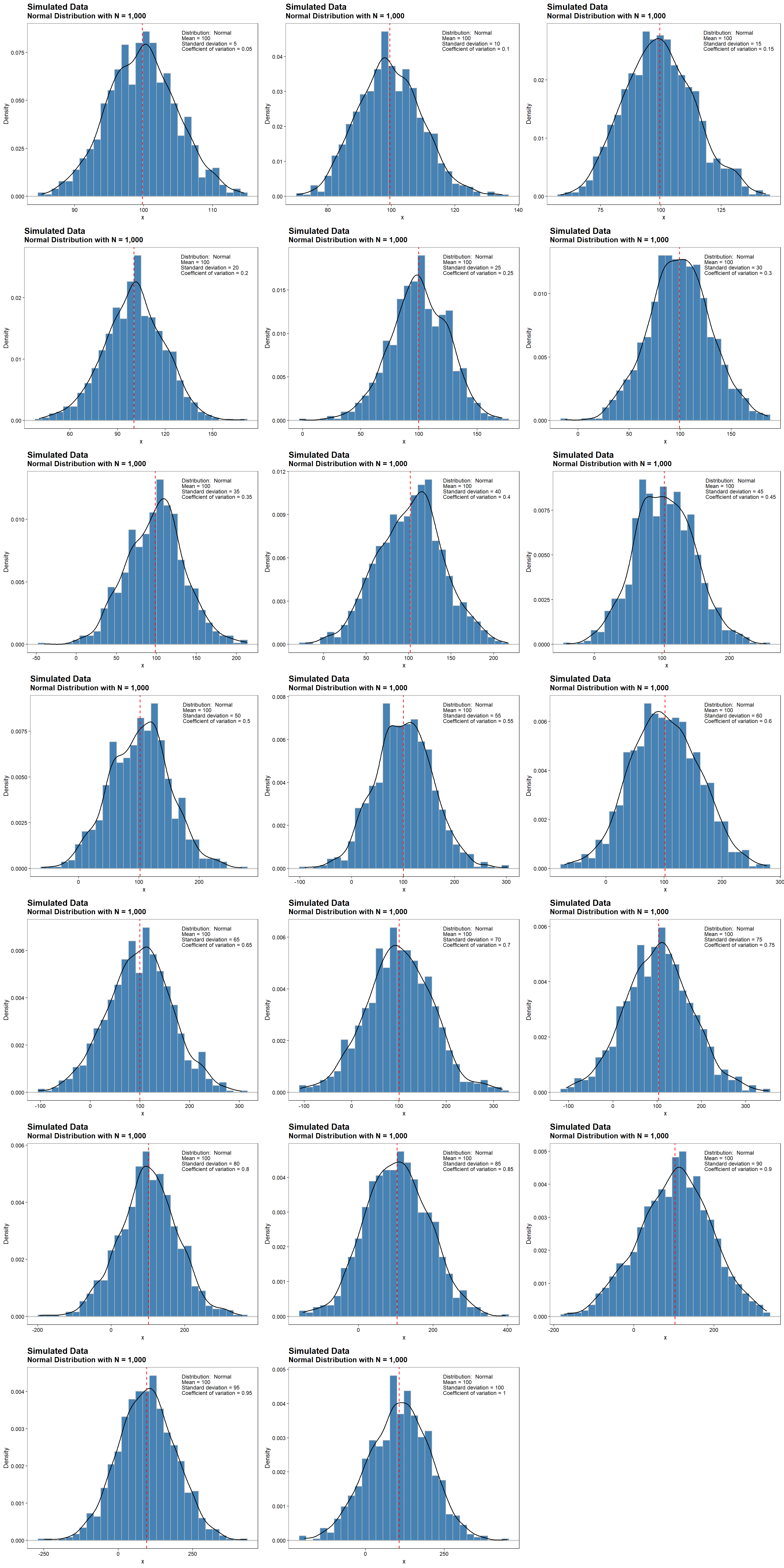
Density plots for normally distributed data with a fixed sample size of 1,000, a mean value of 100, and CV values ranging from 0.05 to 1 are shown below. The dashed, red line represents the mean value of 100. For a normal distribution, there is more dispersion around the mean and the tails become heavier with increasing CV.

plots <- densityplots(Mean = Mean, cv = cv, dist = 'norm')
cowplot::plot_grid(plotlist = plots, ncol = 3)

Power curves for the simulation results for N2 sample sizes ranging from 5 to 100 and assuming a normal distribution are shown below.

# Set distribution (norm, tnorm, or lnorm)
dist <- 'norm'

# Run simulations for all variables
if (ncores <= 1) {
  if (!is.null(set.seed)) set.seed(seed)
  powers <- apply(param, 1, simulation)
} else {
  cl <- parallel::makeCluster(ncores)
  parallel::clusterExport(
    cl,
    list(
      'dist', 'alpha', 'simreps', 'randreps', 'rlnormAlt',
      'rnormt', 'get_data', 'wilcox.test', 't.test',
      'twoSamplePermutationTestLocation')
  )
  if (!is.null(seed)) parallel::clusterSetRNGStream(cl, seed)
  powers <- parallel::parApply(cl, param, 1, simulation)
  parallel::stopCluster(cl)
}

# Convert list of lists to data frame
powers_df <- do.call(rbind, lapply(powers, as.data.frame))

# Combine output with param
param <- bind_cols(param, powers_df)

# Change from wide to long
param_long <- param %>%
  tidyr::gather(test.type, pval, wrs.power:perm.power) %>%
  mutate(
    test.type = factor(
      test.type,
      levels = c('ttest.power', 'wrs.power', 'perm.power')
    )
  )

# Get plot list
plots <- powerplots(param_long)

# Create plot grid
prow <- cowplot::plot_grid(plotlist = plots, ncol = 3)

# Extract legend from first plot
legend <- cowplot::get_legend(
  plots[[1]] + 
    guides(color = guide_legend(nrow = 1)) +
    theme(legend.position = 'bottom')
)

# Add legend underneath plot grid giving it 10% height of one plot
cowplot::plot_grid(prow, legend, ncol = 1, rel_heights = c(1, 0.1))

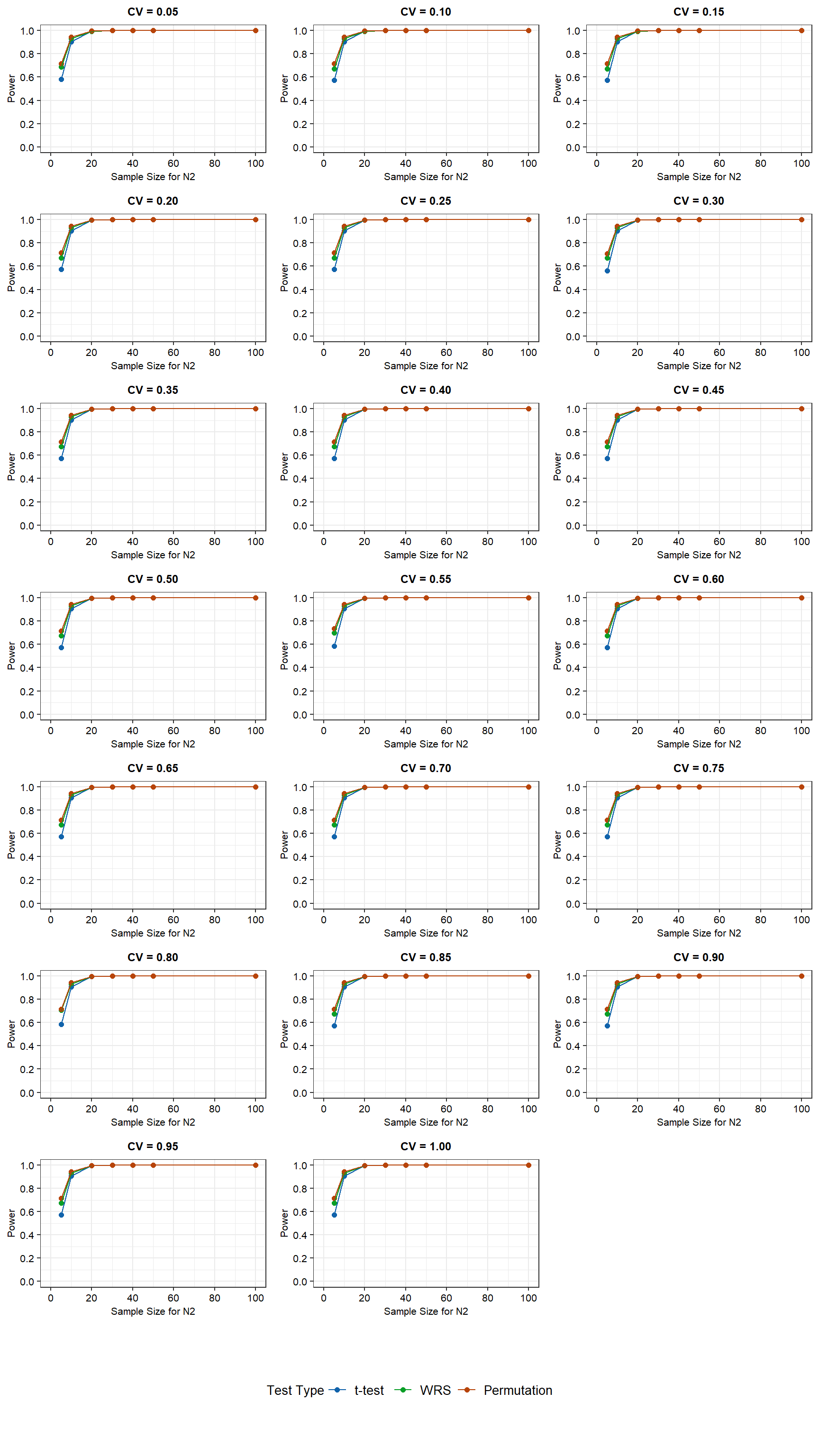
For the normally distributed data with equal variance, the WRS test and the permutation test have more power than the t-test at low N2 sample sizes (less than about 10 observations). The difference in power between the t-test and the other two tests becomes negiglible as the N2 sample size is increased to 10. For a N2 sample size of 20 or more, the power is equivalent for all three tests. For a N2 sample size of 5, power ranges between 60% and 70%, with the lowest power being associated with the t-test. For a N2 sample size of 10, power is approximately 90% for all three tests. CV values between 0.05 and 1 have negigible affect on the power of the tests.

Truncated Normal Distribution

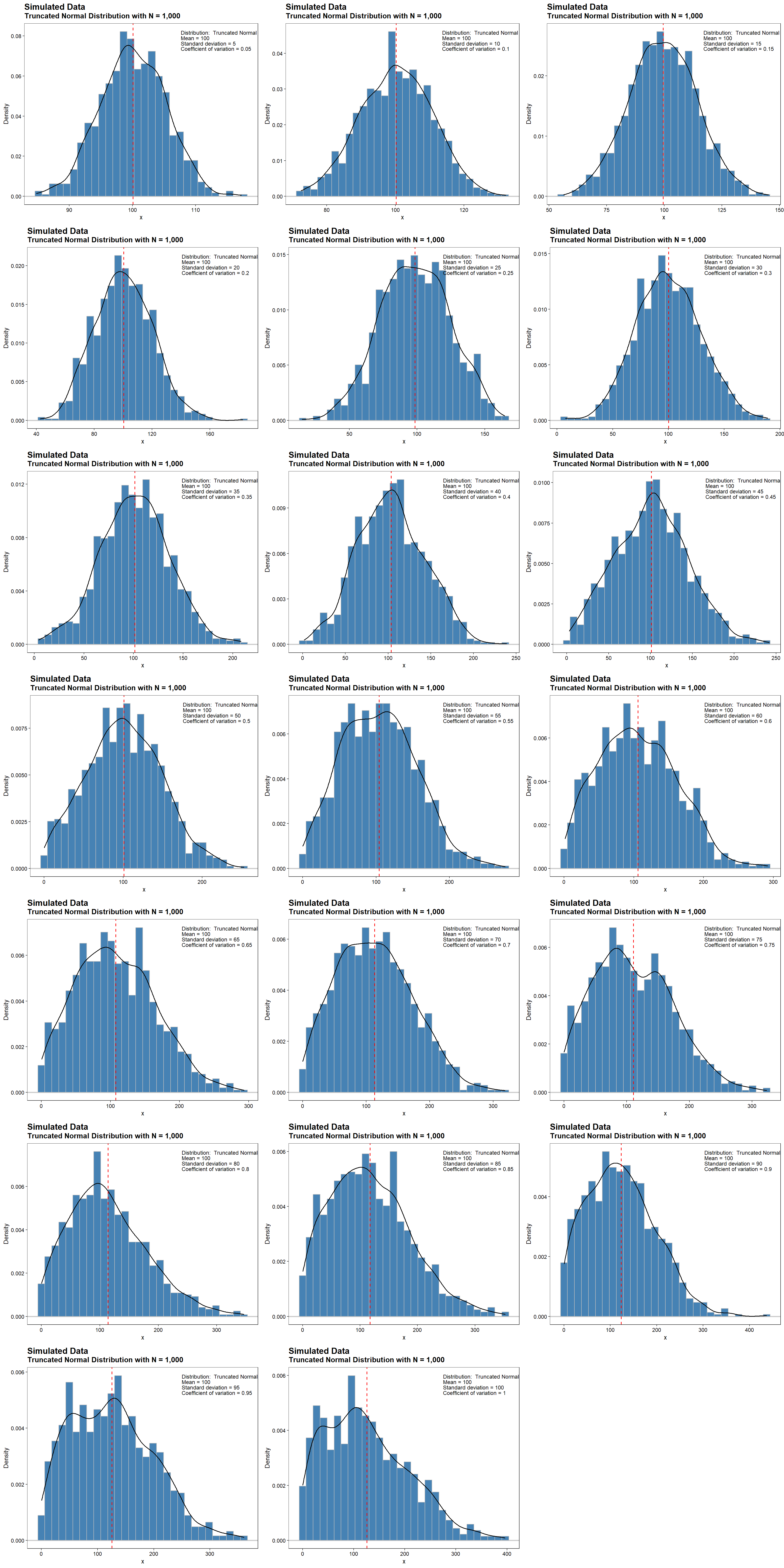
The truncated normal distribution is the probability distribution derived from that of a normally distributed random variable by bounding the random variable from either below or above (or both). For this study, truncation is set below at a value of zero. This provides a mathematically defensible way to preserve the main features of the normal distribution while avoiding negative values. Density plots for truncated normally distributed data with a fixed sample size of 1,000, a mean value of 100, and CV values ranging from 0.05 to 1 are shown below. The dashed, red line represents the mean value of 100. At low values of the CV, the truncated distributions are similar to a normal distribution that is symmetrical around its mean. At higher CV values, the affect of truncation is more pronounced.

plots <- densityplots(Mean = Mean, cv = cv, dist = 'tnorm')
cowplot::plot_grid(plotlist = plots, ncol = 3)

Power curves for the simulation results for N2 sample sizes ranging from 5 to 100 and assuming a truncated normal distribution are shown below.

# Set distribution (norm, tnorm, or lnorm)
dist <- 'tnorm'

# Run simulations for all variables
if (ncores <= 1) {
  if (!is.null(set.seed)) set.seed(seed)
  powers <- apply(param, 1, simulation)
} else {
  cl <- parallel::makeCluster(ncores)
  parallel::clusterExport(
    cl,
    list(
      'dist', 'alpha', 'simreps', 'randreps', 'rlnormAlt',
      'rnormt', 'get_data', 'wilcox.test', 't.test',
      'twoSamplePermutationTestLocation')
  )
  if (!is.null(seed)) parallel::clusterSetRNGStream(cl, seed)
  powers <- parallel::parApply(cl, param, 1, simulation)
  parallel::stopCluster(cl)
}

# Convert list of lists to data frame
powers_df <- do.call(rbind, lapply(powers, as.data.frame))

# Combine output with param
param <- bind_cols(param, powers_df)

# Change from wide to long
param_long <- param %>%
  tidyr::gather(test.type, pval, wrs.power:perm.power) %>%
  mutate(
    test.type = factor(
      test.type,
      levels = c('ttest.power', 'wrs.power', 'perm.power')
    )
  )

# Get plot list
plots <- powerplots(param_long)

# Create plot grid
prow <- cowplot::plot_grid(plotlist = plots, ncol = 3)

# Extract legend from first plot
legend <- cowplot::get_legend(
  plots[[1]] + 
    guides(color = guide_legend(nrow = 1)) +
    theme(legend.position = 'bottom')
)

# Add legend underneath plot grid giving it 10% height of one plot
cowplot::plot_grid(prow, legend, ncol = 1, rel_heights = c(1, 0.1))

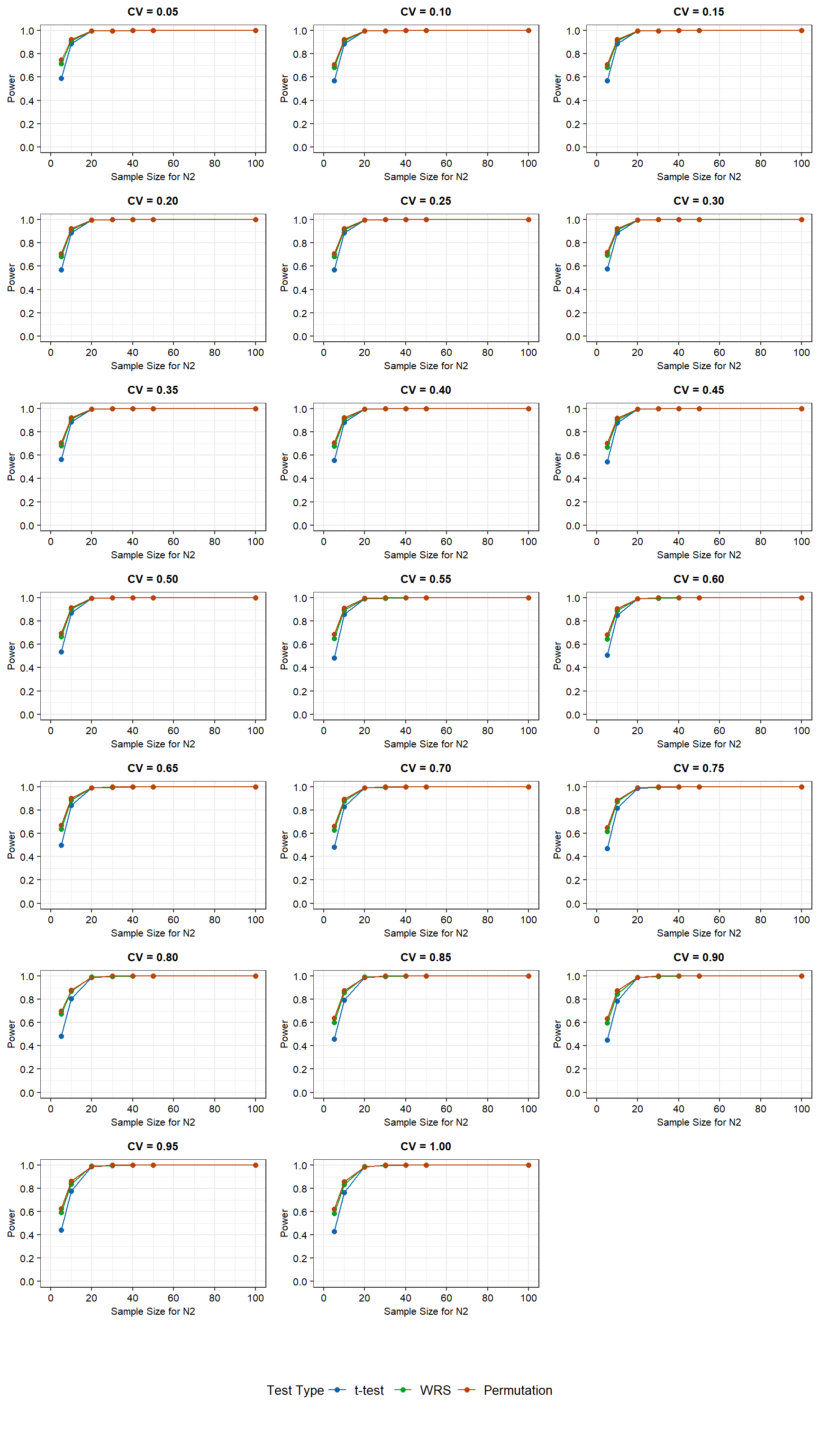
For the truncated normally distributed data with equal variances, the WRS test and the permutation test have more power than the t-test at low N2 sample sizes (less than about 20 observations). Similar to the normal distribution, the difference in power between the t-test and the other two tests becomes negligible as the N2 sample size is increased to 10. For a N2 sample size of 20 or more, the power is equivalent for all three tests. However, contrary to the normal distribution, CV does affect the power of all three tests. Power is highest at low CV values and decreases with increasing CV values for N2 sample sizes below 20. For a sample size of 5, the power of the WRS and permutation tests decreases from approximately 70% to 60% as the CV increases from 0.05 to 1. For these same conditions, the power of the t-test decreases from approximately 60% to 40%. For a sample size of 10, power decreases from approximately 90% to slighly less than 80% as the CV increases from 0.05 to 1. The lowest power is associated with the t-test.

Lognormal Distribution

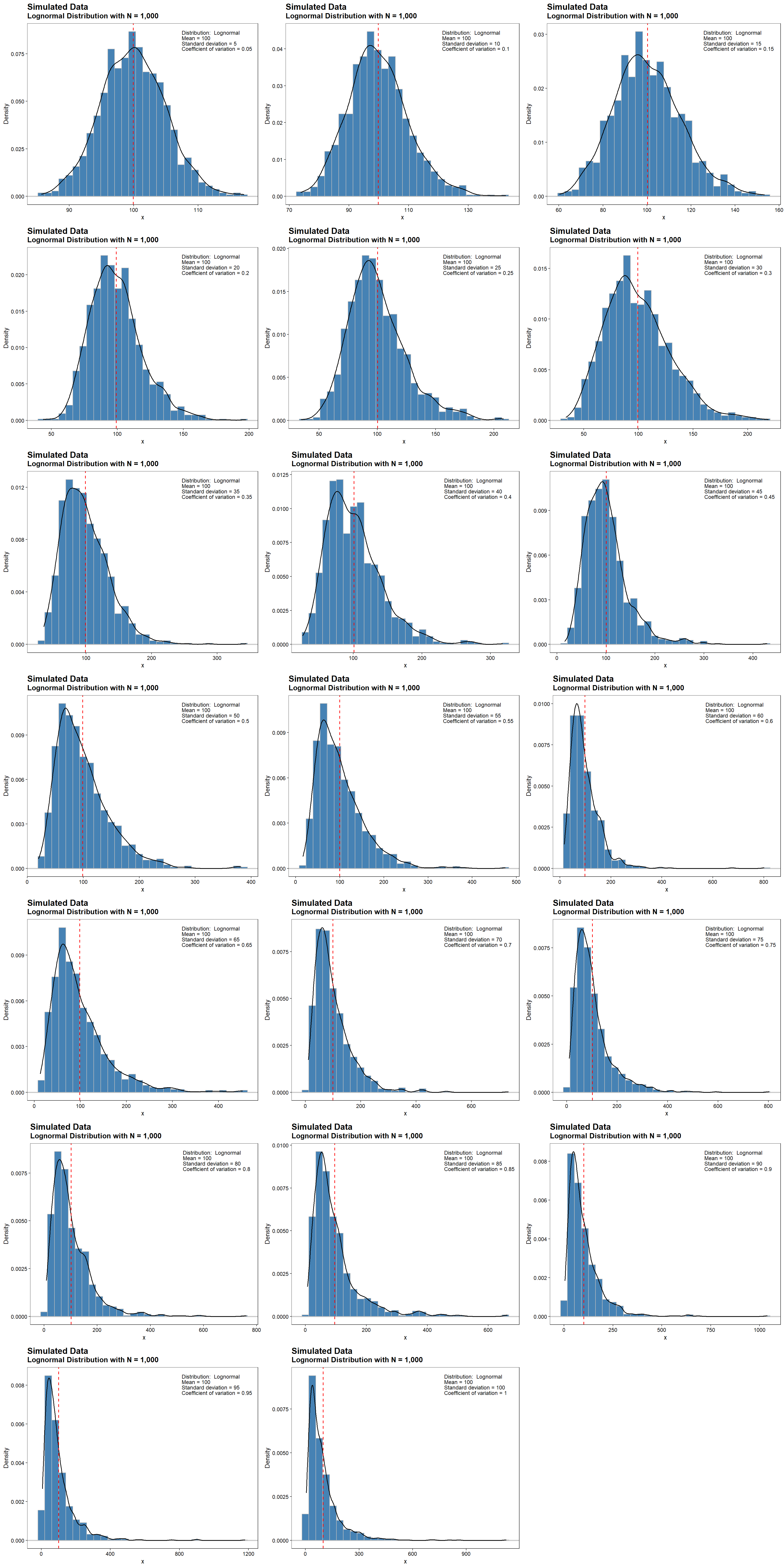
When dealing with data that do not contain negative values or are otherwise skewed, the normality assumption is not satisfied. In this case, a lognormal distribution may better represent the data than the normal distribution. Density plots for lognormally distributed data with a fixed sample size of 1,000, a mean value of 100, and CV values ranging from 0.05 to 1 are shown below. The dashed, red line represents the mean value of 100. At low CV values, where the mean is much larger than the standard deviation, both normal and lognormal distributions fit the data. At higher values of the CV, lognormal distributions are positively skewed with long right tails due to low mean values and high standard deviations.

plots <- densityplots(Mean = Mean, cv = cv, dist = 'lnorm')
cowplot::plot_grid(plotlist = plots, ncol = 3)

Power curves for the simulation results for N2 sample sizes ranging from 5 to 100 and assuming a lognormal distribution are shown below.

# Set distribution (norm, tnorm, or lnorm)
dist <- 'lnorm'

# Run simulations for all variables
if (ncores <= 1) {
 if (!is.null(set.seed)) set.seed(seed)
 powers <- apply(param, 1, simulation)
} else {
 cl <- parallel::makeCluster(ncores)
 parallel::clusterExport(
  cl,
  list(
   'dist', 'alpha', 'simreps', 'randreps', 'rlnormAlt',
   'rnormt', 'get_data', 'wilcox.test', 't.test',
   'twoSamplePermutationTestLocation')
 )
 if (!is.null(seed)) parallel::clusterSetRNGStream(cl, seed)
 powers <- parallel::parApply(cl, param, 1, simulation)
 parallel::stopCluster(cl)
}

# Convert list of lists to data frame
powers_df <- do.call(rbind, lapply(powers, as.data.frame))

# Combine output with param
param <- bind_cols(param, powers_df)

# Change from wide to long
param_long <- param %>%
 tidyr::gather(test.type, pval, wrs.power:perm.power) %>%
 mutate(
  test.type = factor(
   test.type,
   levels = c('ttest.power', 'wrs.power', 'perm.power')
  )
 )

# Get plot list
plots <- powerplots(param_long)

# Create plot grid
prow <- cowplot::plot_grid(plotlist = plots, ncol = 3)

# Extract legend from first plot
legend <- cowplot::get_legend(
 plots[[1]] + 
  guides(color = guide_legend(nrow = 1)) +
  theme(legend.position = 'bottom')
)

# Add legend underneath plot grid giving it 10% height of one plot
cowplot::plot_grid(prow, legend, ncol = 1, rel_heights = c(1, 0.1))

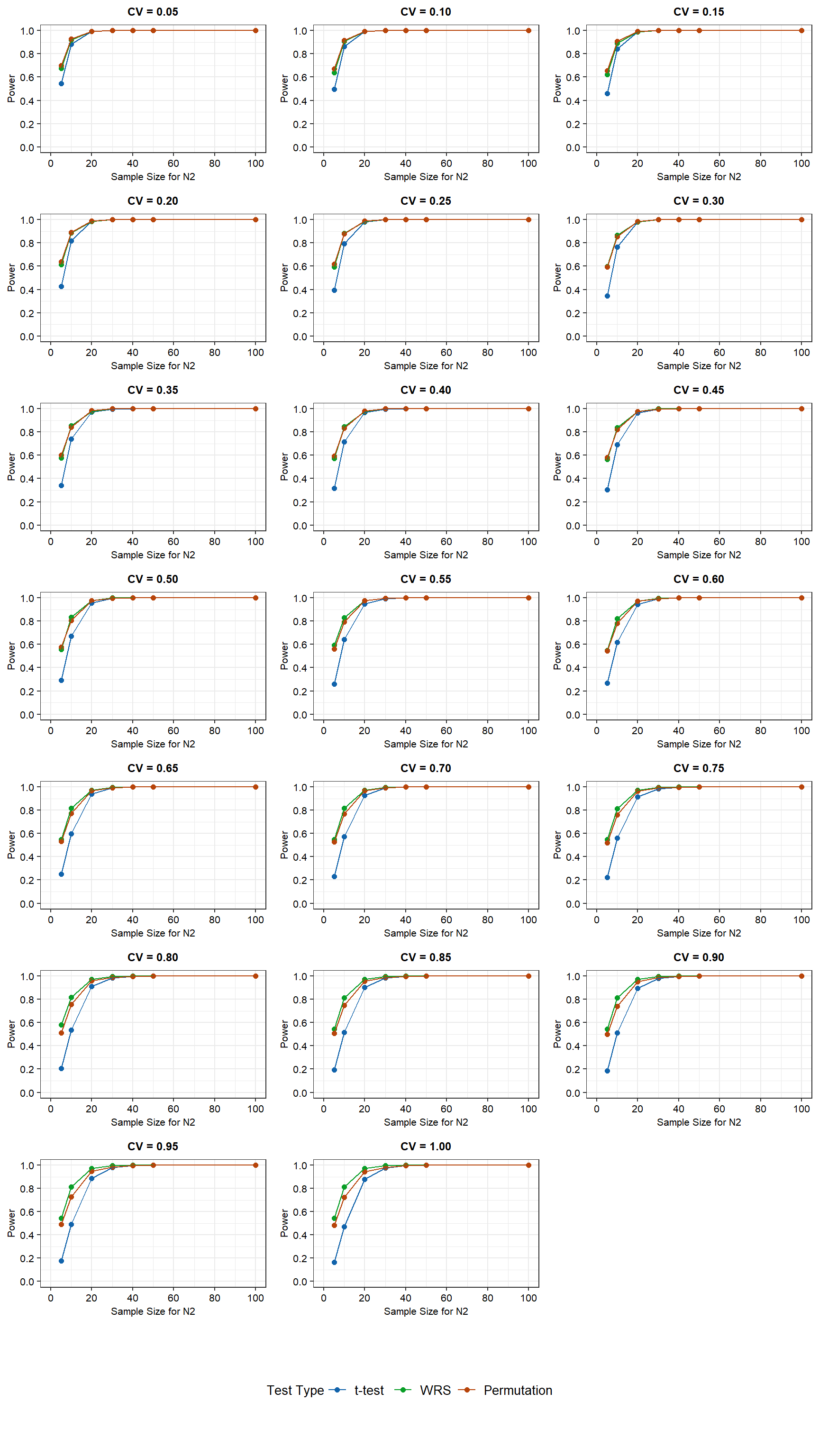
For the lognormally distributed data with equal variances, the WRS test and the permutation test have more power than the t-test at low N2 sample sizes. The difference in power between the t-test and the other two tests becomes smaller as the N2 sample size is increased and depends on the CV. The t-test requires a N2 sample size of 20 or more to match the power of the other two tests when the CV is 0.5 or less. At higher CV values, the t-test requires a sample size of 30 or more for equivalent power. For N2 sample sizes of 30 or more, power is independent of CV. For N2 sample sizes of less than 30, power decreases with increasing CV. For a N2 sample size of 5, the power of the WRS and permutation tests decreases from approximately 70% to 50% as CV increases from 0.05 to 1. For these same conditions, the power of the t-test decreases from approximately 55% to less than 20%. For a N2 sample size of 10, the power of the WRS and permutation tests decreases from approximately 90% to 70% as CV increases from 0.05 to 1. The lowest power is associated with the permutation test. For a N2 sample size of 10, the power of the t-test decreases from slightly less than 90% to almost 50% as CV increases from 0.05 to 1.

Conclusions

Statistical tests require the careful formulation of a null hypothesis and an alternative hypothesis. Many of the classical statistical tests build on statistical assumptions concerning the data. Regardless of distribution type, the power of the two-sample tests increases with N2 sample size and generally decreases with CV. Under the conditions evaluated and for small N2 sample sizes, the nonparametric WRS test and the permutation test have more power than the parametric t-test, even when data are normally distributed. For N2 sample sizes of 30 or more, the power of all three tests are comparable. Except for lognormally data with CV values close to 1, there is little difference between the power of the WRS test and the permutation test. For lognormally data with CV values close to 1, the WRS test has more power than the permutation test.

The purpose of this study was to compare the performance of two-sample hypothesis tests when groups have unequal sample sizes. The parameters used in this study provide reference points that may not emulate all conditions encountered. Nevertheless, the results presented here provide useful information for consideration when designing or conducting hypothesis tests for two, independent groups of data with vastly different sample sizes.

References

Good, P.I. 2005. Resampling Methods: A Practical Guide to Data Analysis. Third Edition. Birkhauser, Boston.

Lehmann E.L. and J.P. Romano. 2005. Testing Statistical Hypothesis Third Edition. Springer, New York.

Mann H.B. and D.R. Whitney. 1947. On a test of whether one of two random variables is stochastically larger than the other.* Annals of Mathematical Statistics*, 18:50-60.

Wilcoxon, F. 1945. Individual comparisons by ranking methods. Biometrics, 1:80-83.