Introduction

Correlation analysis is a statistical method that is used to quantify the direction and strength of a relationship between two variables. Generally, for small sample sizes, the calculated magnitude of a correlation is unstable. With increasing sample size, the sample correlation approaches the true value with a continuously decreasing confidence interval. It is technically possible to calculate confidence intervals with very small samples, but the corresponding confidence intervals will include a wide range of values because the standard errors will be quite large. The necessary sample size to achieve stable estimates for correlations depends on the effect size, the width of the corridor of stability (i.e., the acceptable confidence interval around the true value where deviations are tolerated), and the requested confidence that the correlation is within the corridor of stability.

Background

Correlation tests are arguably one of the most commonly used statistical procedures, and are used to assess relationships among variables. Correlation is a statistical measure that describes how two variables are related and indicates that as one variable changes in value, the other variable tends to change in a specific direction. The strength of the association or dependence between two variables, how predictably they covary, is measured by a correlation coefficient. Correlation coefficients can take on values between +1 and -1. When there is no correlation between two variables, correlation is equal to zero. When one variable increases as the second increases, correlation is positive. When the variables vary together but in opposite directions, correlation is negative. Although correlation measures observed covariation between two variables, that is, how one varies by the other, it does not provide evidence for causal relation between the two variables.

Three commonly used measures of correlation are Pearson’s product-moment correlation or Pearson’s r, Spearman’s rho, and Kendall’s tau. These three measure of correlation are summarized as follows:

Pearson’s r: This is the most common measure of correlation. It is used to measure strength and direction of a linear relationship between two variables. Mathematically, this can be done by dividing the covariance of the two variables by the product of their standard deviations. It is a parametric test that is only recommended when the relationship between the two variables is linear. Pearson’s correlation assumes normality of the data (for statistical inference), equal variances, and no outlying observations.

Spearman’s rho: This is a non-parametric measure of correlation between two variables and is equivalent to the Pearson correlation between the rank scores of those two variables. While Pearson’s correlation assesses linear relationships, Spearman’s sho assesses monotonic relationships (whether linear or not). Because Spearman’s rho depends only on the ranks of the data and not the observations themselves, it is resistant to outliers and can be implemented even in cases where some of the data are censored, such as concentrations known only as less than an analytical detection limit.

Kendall’s tau: Much like Spearman’s rho, Kendall’s tau is a rank-based procedure that measures the strength of the monotonic relationship between two variables. Because it depends only on the ranks of the data and not the observations themselves, it can be implemented in cases where some of the data are categorical. One advantage of Kendall’s tau is that it can be adapted for use with censored data containing multiple detection or reporting limits. In general, Kendall’s tau will be lower than values of Pearson’s r for linear associations for any given linearly related data. Strong linear correlations of r = 0.9 (or above) typically correspond to tau values of about 0.7 (or above). These lower values do not mean that Kendall’s tau is less sensitive than Pearson’s r, but simply that a different scale of correlation is being used.

Depending on sample size, Spearman’s rho is relatively similar in terms of power to Pearson’s r with normally distributed data, and is far superior with even slight departures from normality. Generally, Spearman’s rho is more powerful than Pearson’s r across a range of nonnormal bivariate distributions. Spearman’s rho provides accurate estimates of the true correlations for normally and non-normally distributed data with no or minimal loss of power and adequate control over the false positive rate. When the data contain censored results with multiple detection or reporting limits, Kendall’s tau is considered the most appropriate test for correlation.

Sample Size Based on Null Hypothesis

The sample size required to determine whether a correlation coefficient differs from zero can be determined using the pwr package develped for R by Stephane Champely. The function pwr.r.test() can compute power of the test or determine parameters required to obtain a target power for Pearson’s r. Arguments for pwr.r.test() include:

• n = number of observations
• r = linear correlation coefficient
• sig.level = significance level (Type I error probability)
• power = power of test (1 minus Type II error probability)
• alternative = string specifying the alternative hypothesis, must be one of “two.sided” (default), “greater”, or “less”

By specifying n = NULL in the arguments to pwr.r.test(), the function calcuates the sample size based on the other arguments. Let’s determine the sample size for a linear correlation of 0.5 at a significanve level of 0.05 with 80% power.

# Load library
library(pwr)

# Detemine sample size for specified variables
r <- 0.5
sig <-0.05
power <- 0.8
p.out <- pwr.r.test(
  n = NULL,
  r = r,
  sig.level = sig,
  power = power,
  alternative = 'two.sided'
)
p.out
## 
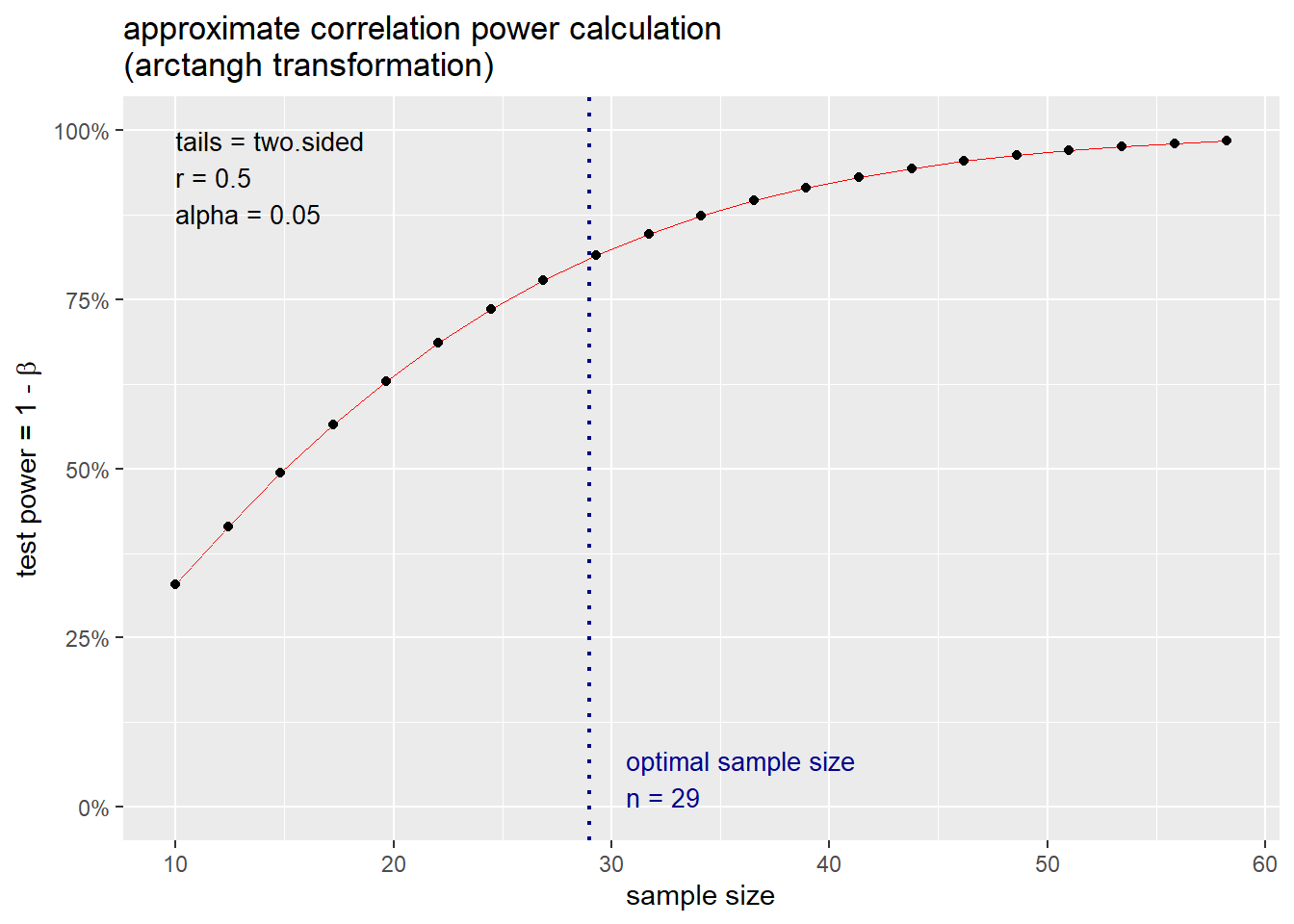
##      approximate correlation power calculation (arctangh transformation) 
## 
##               n = 28.24841
##               r = 0.5
##       sig.level = 0.05
##           power = 0.8
##     alternative = two.sided

The results indicate that 29 samples are required to have an 80% chance of correctly rejecting the null hypothesis of r = 0 at the 0.05 significance level assuming a linear correlation of 0.5.

The pwr package provides a generic plot function that shows power change as a function of sample size. Let’s plot the power change as a function of sample size for our example.

# Get plot of optimal sample size
plot(p.out)

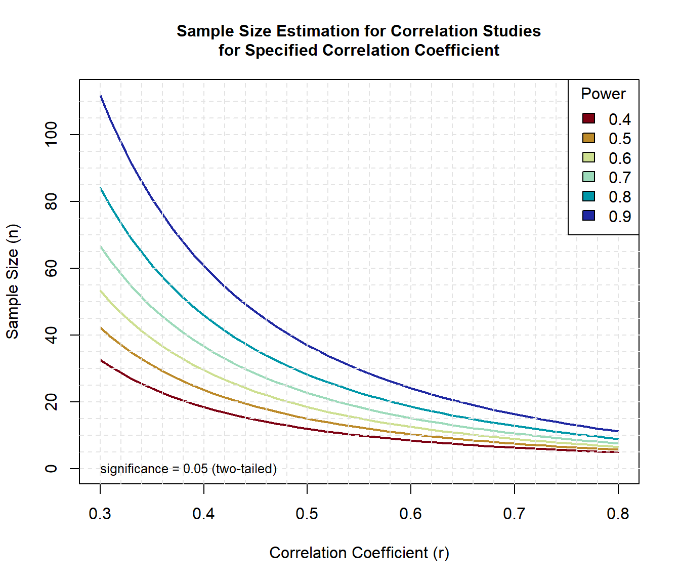
Let’s use the functions in the pwr package to generate sample size curves for detecting correlations of various sizes for different levels of power.

# Create range of correlations
r <- seq(0.3, 0.8, 0.01)
nr <- length(r)

# Create range of power values
p <- seq(0.4, 0.9, 0.1)
np <- length(p)

# Obtain sample sizes
samsize <- array(numeric(nr*np), dim = c(nr, np))
for (i in 1:np){
  for (j in 1:nr){
    result <- pwr.r.test(
      n = NULL, r = r[j],
      sig.level = 0.05, power = p[i],
      alternative = 'two.sided'
    )
    samsize[j,i] <- result$n   # ceiling(result$n)
  }
}

# Set ranges and colors for graph
xrange <- range(r)
#yrange <- round(range(samsize))
yrange <- c(0, round(max(samsize)))
#colors <- rainbow(length(p))
colors <- hcl.colors(length(p), 'Roma')

# Setup graph
plot(
  xrange, yrange, type = 'n',
  xlab = 'Correlation Coefficient (r)',
  ylab = 'Sample Size (n)'
)

# Add power curves
for (i in 1:np){
  lines(r, samsize[,i], type = 'l', lwd = 2, col = colors[i])
}

# Add annotation (grid lines, title, legend)
abline(v = 0, h = seq(0, yrange[2], 5), lty = 2, col = 'grey89')
abline(h = 0, v = seq(xrange[1], xrange[2], 0.02), lty = 2, col = 'grey89')
title(
  main = c(
    'Sample Size Estimation for Correlation Studies',
    'for Specified Correlation Coefficient'
  ),
  cex.main = 1
)
text(
  x = 0.3, y = 0, adj = 0,
  label = 'significance = 0.05 (two-tailed)',
  cex = 0.8
)
legend('topright', title = 'Power', as.character(p), fill = colors)

Sample Size Based on Confidence Interval

Although the value of the correlation is not influenced by the number of data points, the confidence interval of the correlation is strictly dictated by the size of the data set and the chosen level of confidence. Consider, for example, a correlation of r = 0.5 with a sample size of 20. This correlation is significantly different from zero (two-tailed p-value of 0.047). Hence, it might be concluded with some confidence that the correlation is significantly greater than zero. However, plausible values of the true correlation, as expressed by a 95% confidence interval, range from 0.06 to 0.78. The estimate is quite unsatisfactory from an accuracy point of view. Is the true correlation equal to 0.06, which would be regarded as a very small effect, or 0.78, which would be regarded as a large effect in many contexts?

A 95% confidence interval is an interval that, if constructed in a large number of samples, should cover the true population parameter in 95% of those samples. The use of confidence intervals can mitigate some of the limitations of null hypothesis significance testing. Confidence intervals reduce the mistake of accepting the null hypothesis for a nonsignificant test result. Confidence intervals shift focus toward the continuous dimension of effect size rather than the simple binary dimension of significant versus nonsignificant, and they highlight the idea that estimates of effect size are always uncertain. Because of the advantages of using confidence intervals, accurate construction of such intervals is important.

The presize package can be used to calcuate the width of the confidence interval for a given sample size, correlation, and confidence level. The prec_cor() function returns the sample size or the precision for a given Pearson, Spearman, or Kendall correlation coefficient. Let’s calculate the confidence internal for our example where the linear correlation is 0.5 and the sample size is 29.

# load library
library(presize)

# Pearson correlation coefficient
prec_cor(
  r = 0.5, n = 29,
  conf.level = 0.95,
  method = 'pearson'
)
## 
##      precision for pearson 's correlation coefficient 
## 
##     r  n conf.width conf.level       lwr       upr
## 1 0.5 29  0.5688618       0.95 0.1634463 0.7323081

For a linear correlation of 0.5 and a sample size of 29, the 95% confidence interval for r is [0.16, 0.73]. With a wide interval, such as this, it’s difficult to understand whether there is a meaningful relationship between the variables. The associated confidence interval for a sample size of 29 encloses both effects that are close to zero and large effects, and imparts a degree of uncertainty around the correlation, particularly when it comes to replicability. While this correlation is significant at p < 0.05, it would be worthwhile to collect enough data that improve precision of the main result.

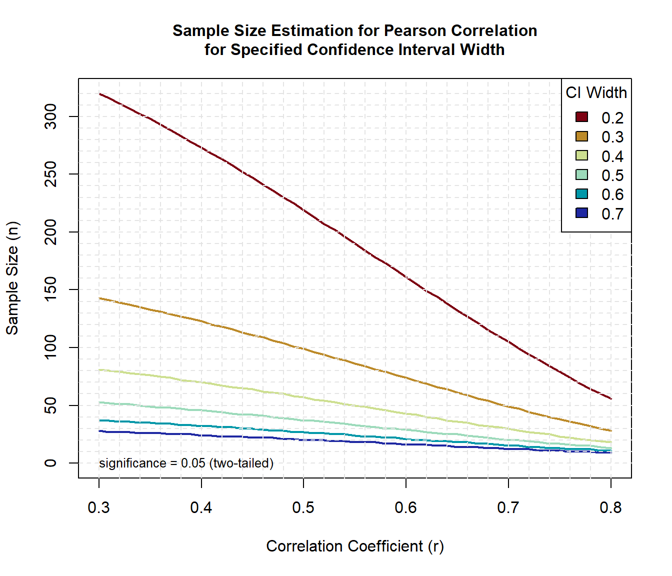
Similar to the null hypothesis method shown above, we can use the functions in the presize package to generate sample size curves for detecting correlations of various sizes for different 95% confidence interval widths.

# Create range of correlations
r <- seq(0.3, 0.8, 0.01)
nr <- length(r)

# Create range of full width values for confidence interval
w <- seq(0.2, 0.7, 0.1)
nw <- length(w)

# Obtain sample sizes
samsize <- array(numeric(nr*nw), dim = c(nr, nw))
for (i in 1:nw){
  for (j in 1:nr){
    result <- prec_cor(
      r = r[j], conf.width = w[i],
      conf.level = 0.95,
      method = 'pearson'
    )
    samsize[j,i] <- result$n   # ceiling(result$n)
  }
}

# Set ranges and colors for graph
xrange <- range(r)
#yrange <- round(range(samsize))
yrange <- c(0, round(max(samsize)))
#colors <- rainbow(length(w))
colors <- hcl.colors(length(w), 'Roma')

# Setup graph
plot(
  xrange, yrange, type = 'n',
  xlab = 'Correlation Coefficient (r)',
  ylab = 'Sample Size (n)'
)

# Add power curves
for (i in 1:nw){
  lines(r, samsize[,i], type = 'l', lwd = 2, col = colors[i])
}

# Add annotation (grid lines, title, legend)
abline(v = 0, h = seq(0, yrange[2], 10), lty = 2, col = 'grey89')
abline(h = 0, v = seq(xrange[1], xrange[2], 0.02), lty = 2, col = 'grey89')
title(
  main = c(
    'Sample Size Estimation for Pearson Correlation',
    'for Specified Confidence Interval Width'
  ),
  cex.main = 1
)
text(
  x = 0.3, y = 0, adj = 0,
  label = 'significance = 0.05 (two-tailed)',
  cex = 0.8
)
legend('topright', title = 'CI Width', as.character(w), fill = colors)

Now, let’s plot the confidence interval for a Pearson correlation of 0.5.

# Set correlation coefficient
r <- 0.5

# Create range of sample sizes
s <- seq(1, 500, 1)
ns <- length(s)

# Obtain confidence intervals for the sample sizes
lwr <- NULL
upr <- NULL
for (j in 1:ns){
  result <- prec_cor(
    r = 0.5, n = s[j],
    conf.level = 0.95,
    method = 'pearson'
  )
  lwr[j] <- result$lwr
  upr[j] <- result$upr
}

# Setup ranges for graph
xrange <- c(0, round(max(s)))
yrange <- c(-1, 1)

# Setup graph
plot(
  xrange, yrange, type = 'n',
  xlab = 'Sample Size (n)',
  ylab = 'Correlation Coefficient (r)'
)
lines(s, lwr, type = 'l', lwd = 2, col = 'black')
lines(s, upr, type = 'l', lwd = 2, col = 'black')

# Add annotation (grid lines, title, legend)
abline(v = 0, h = seq(-1, yrange[2], 0.1), lty = 2, col = 'grey89')
abline(h = 0, v = seq(0, xrange[2], 20), lty = 2, col = 'grey89')
title(
  main = c(
    '95% Confidence Interval for Pearson Correlation',
    'for Correlation Coefficient of 0.5'
  ),
  cex.main = 1
)
text(
  x = 270, y = -0.9, adj = 0,
  label = 'Confidence interval calculated according\n to Bonett and Wright (2000)',
  cex = 0.8
)

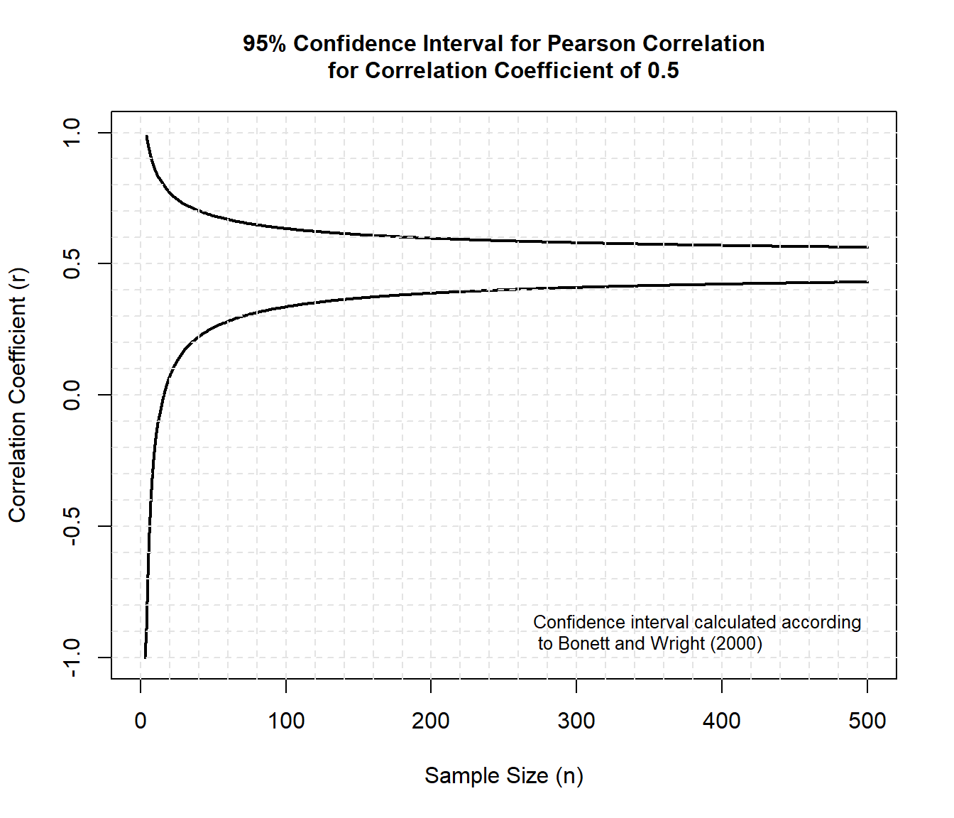
When the sample size is large, the error is lower and the sample correlation converges to the population parameter. The sampling error is higher for small sample sizes and because of this we have a higher probability that an error will be made when estimating the population parameter.

As an example, let’s generate two random normal variables with 1,000,000 cases and correlation of 0.5 that represent the population. We will use the laxyCov() function of the rockchalk package. The rockchalk package includes a collection of functions for interpretation and presentation of regression analysis. The laxyCov() function is a flexible function that allows the creation of a covariance matrix. It’s lazy because the correlation and standard deviation infomation may be supplied in a variety of formats.

# Load libraries
library(rockchalk)
library(ggplot2)

# Set seed for reproducibility
set.seed(12345)

# Define covariance matrix for two variables with sd = 20 and correlation 0.5
myCov <- lazyCov(Rho = 0.5, Sd = 20, d = 2)

# Create two variables with specified covariance matrix and
# M = 100 --> Population = 1,000,000
myData <- data.frame(mvrnorm(n = 1000000, mu = c(100, 100), Sigma = myCov))
 
# Calculate population correlation
pop_cor <- cor(myData[,1], myData[,2])

Let’s create 1,000 samples that go from 5 to 5,000 in steps of 5 (5, 10, 15, 20…) and for each sample calculate the correlation between the two variables and the absolute deviation of the sample correlation from the population correlation.

# Create dataframe for saving the results
rez <- data.frame()

for (i in (1:1000)) {
  sampleData <- myData[sample(nrow(myData), i*5),]
  q <- cor(sampleData$X1,sampleData$X2, method = 'pearson')
  rez[i,1] <- i*5             # sample size - V1
  rez[i,2] <- q               # sample correlation - V2
  rez[i,3] <- abs(q-pop_cor)  # absolute deviation from population correlation - V3
}

Now, let’s plot the sample correlation as a function of sample size.

# Plot correlation and sample size
xrange <- c(0, max(rez[,1]))
yrange <- range(rez[,2])
with(rez,
  plot(
    xrange, yrange, type = 'n',
    xlab = 'Sample Size (n)',
    ylab = 'Correlation Coefficient (r)'
  )
)

# Add grid lines
abline(v = 0, h = seq(-1, yrange[2], 0.05), lty = 2, col = 'grey89')
abline(h = 0, v = seq(0, 5000, 200), lty = 2, col = 'grey89')

# Add points
with(rez, points(V1, V2, pch = 20, cex = 1))

# Add annotation
title(
  main = c(
    'Pearson Correlation as a Function of Sample Size',
    'for Correlation Coefficient of 0.5'
  ),
  cex.main = 1
)
text(
  x = 3500, y = 0.88, adj = 0,
  label = paste('Population r = ', round(pop_cor, 3)),
  cex = 1
)
text(
  x = 3000, y = 0, adj = 0,
  label = 'Sampling error is higher for small\nsample sizes.',
  cex = 0.8
)

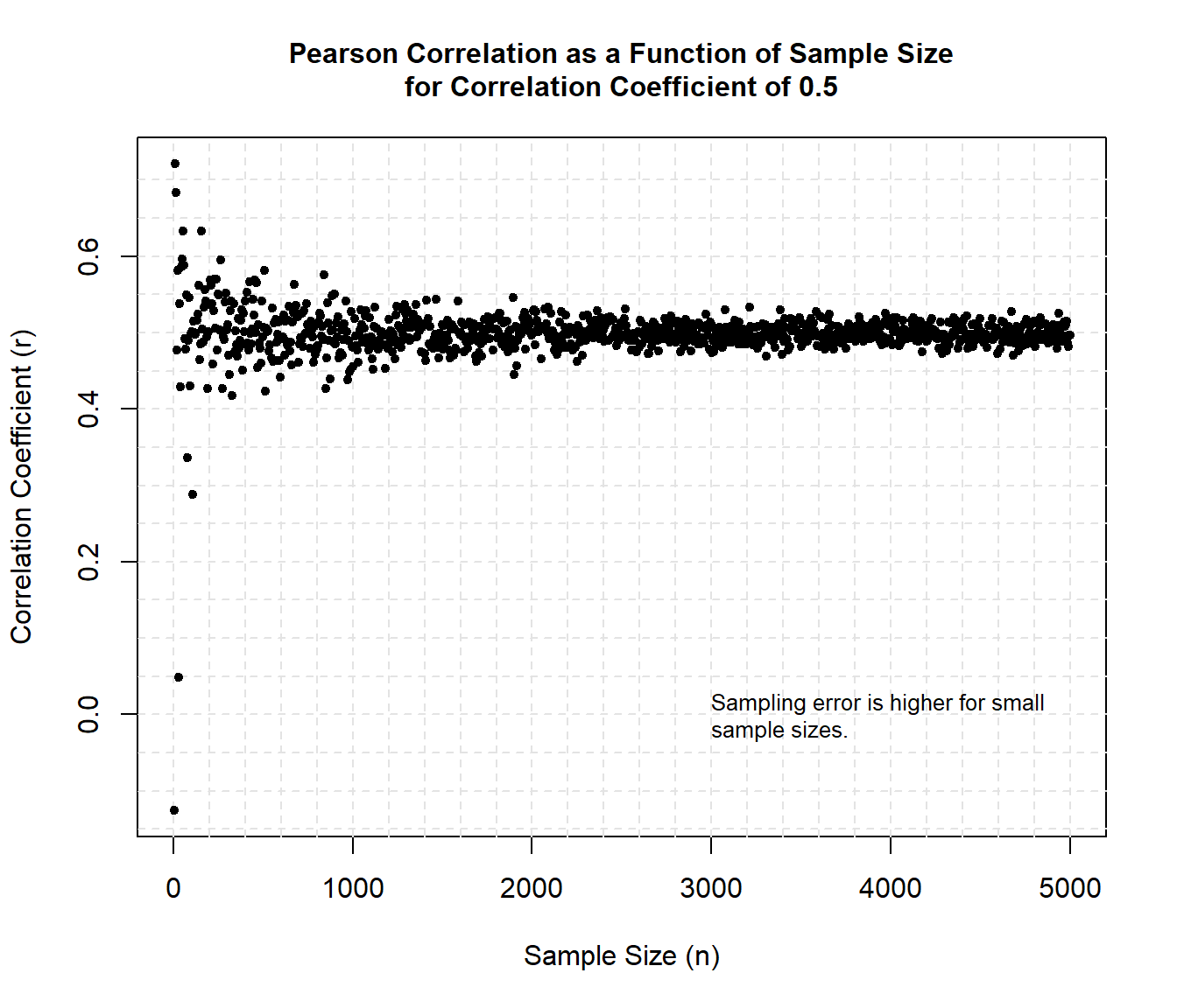
Sample correlations converge to the population value with increasing sample size, but the estimates are unstable in small samples. Minor fluctuations around the true value most likely can be tolerated, but large deviations could be deemed more problematic, depending on the research setting.

Another way to illustrate the effect of sample size on the estimate of correlation is to plot the absolute deviation of the sample correlations from the population correlation.

xrange <- c(0, max(rez[,1]))
yrange <- range(rez[,3])
with(rez,
  plot(
    xrange, yrange, type = 'n',
    xlab = 'Sample Size (n)',
    ylab = 'Absolution Deviation'
  )
)

# Add grid lines
abline(v = 0, h = seq(-1, yrange[2], 0.02), lty = 2, col = 'grey89')
abline(h = 0, v = seq(0, 5000, 200), lty = 2, col = 'grey89')

# Add points
with(rez, points(V1, V3, pch = 20, cex = 1))

# Add annotation
title(
  main = c(
    'Absolute Deviation from Population Correlation',
    'as a Function of Sample Size'
  ),
  cex.main = 1
)
text(
  x = 2900, y = 0.55, adj = 0,
  label = paste(
    'Correlation between the error and the\nsample size is ',
    round(cor(rez$V1,rez$V3), 2)
  ),
  cex = 0.8
)

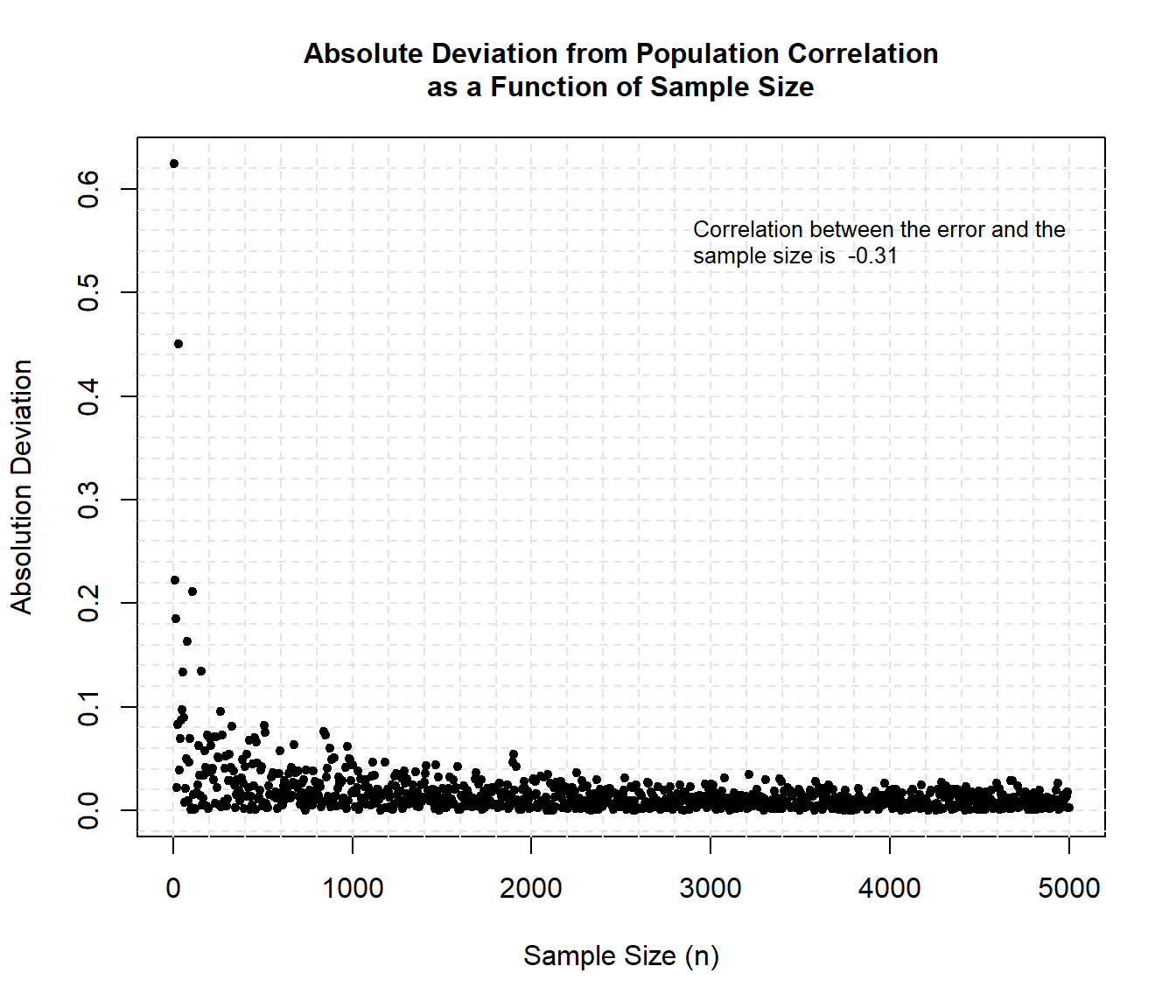
The results show that as sample size increases the error decreases. The correlation between the error and the sample size can be approximated as -0.31.

Conclusion

Determination of the appropriate sample size to use when performing inference for a correlation coefficient is usually based on achieving sufficient power that the test can reject the null hypothesis that the correlation is zero. Sample sizes found using this method can yield confidence intervals that are so wide that they provide very little useful information about the magnitude of the correlation. An alternative approach is to select the sample size based on the desired width of the resulting confidence interval for the correlation. The goal is to choose a sample size that achieves a sufficiently narrow confidence interval for measuring the smallest correlation of potential interest. The sample size to be collected in a study should ideally not only depend on the availability of time and other resources, but also on a careful power analyses.

As a final note, the Pearson correlation can be robust in terms of the point estimate and the Type I error rate, which usually converge on the correct values as the sample size increases. However, the Pearson correlation is not generally robust in terms of confidence intervals or power, even with large samples. Thus, at least for the Pearson correlation, nonnormal data should be approached cautiously and with a careful consideration of alternative methods.