Two-Sample Permutation Test of Difference in Means
By Charles Holbert
December 22, 2022
Introduction
There are a large number of statistical tests that can be used to determine whether the difference between two groups of data is statistically significant. If the data in each group are normally distributed, a two-sample t-test can be used to compare the means of the two groups. If this assumption is severely violated, the nonparametric Wilcoxon Rank Sum (WRS) test, also known as the two-sample Mann-Whitney U test, may be considered instead. This is a nonparametric version of a two-sample t-test and calculates whether the medians of the two distributions are different or similar, assuming observations in each group are identically and independently distributed apart from location. When observations represent very different distributions, the method is a test of dominance between distributions. However, when the interest is in the differences of means, an alternative is a two-sample permutation test.
This post demonstrates how to perform a two-sample permutation test using various packages within the R environment for statistical computing and visualization.
Permutation Tests
Permutation tests are used to test for differences between means for skewed, moderately sized datasets. They compute the p-value using computer-intensive methods rather than assuming data follow normal distributions. Permutation tests are also called resampling methods (Good 2001), randomization tests (Manly 2007), and observation randomization tests (Brown and Rothery 1993). In 1935, R. A. Fisher introduced the idea of a randomization test (Manly 2007; Efron and Tibshirani 1993). Because of the large computing resources needed to enumerate all possible outcomes, especially for large sample sizes, permutation tests did not become popular until around the late 1980s (Helsel et al. 2020).
The two-sample permutation test works by enumerating all possible permutations of group assignments, and for each permutation computing the difference between the measures of location for each group. The measure of location for a group could be the mean, median, or some other measure. Under the null hypothesis, the underlying distributions for each group are the same; therefore, it should make no difference which group an observation gets assigned to. To check whether the null hypothesis can be rejected, the data are randomly shuffled, again and again, and the difference between the two randomly created groups is recorded each time. At the end of the test, the actual difference observed between the two groups is compared with the thousands of simulations performed to see how likely/unlikely it would be under the null hypothesis.
For a one-sided upper alternative, the p-value is computed as the proportion of times that the differences of the means (or medians) in the permutation distribution are greater than or equal to the observed difference in means (or medians). For a one-sided lower alternative hypothesis, the p-value is computed as the proportion of times that the differences in the means (or medians) in the permutation distribution are less than or equal to the observed difference in the means (or medians). For a two-sided alternative hypothesis, the p-value is computed as the proportion of times the absolute values of the differences in the means (or medians) in the permutation distribution are greater than or equal to the absolute value of the observed difference in the means (or medians).
A two-sample permutation test for differences in means avoids the assumptions of the parametric t-test. The t-test requires that the data from each group follow a normal distribution and that the groups have the same variance. Violation of these assumptions leads to a loss of power, raising p-values, and failing to find differences between group means when they occur. The permutation test still assumes, however, that under the null hypothesis, the distributions of the observations from each group are exactly the same, and under the alternative hypothesis there is simply a shift in location (Millard 2013). Thus, the shape and spread of the two distributions should be the same whether the null hypothesis is true or not.
Simulated Data
For this example, let’s generate 20 observations from a lognormal distribution with parameters mean = 10 and cv = 2, and 10 observations from a lognormal distribution with parameters mean = 5 and cv = 2. We will use these data to test the null hypothesis that the mean of group 1 is equal to or less than the mean for group 2 against the alternative that the mean for group 1 is greater than the mean for group 2. To generate the data, we will use the rlnormAlt() function from the EnvStats package.
# Load libraries
library(dplyr)
library(EnvStats)

# Load functions
source('functions/sumstats.R')

# Set seed for reproducibility
set.seed(123)

# Create two data sets
dat1 <- data.frame(
  Result = rlnormAlt(20, mean = 10, cv = 2),
  Censored = FALSE,
  Group = 'Group 1'
)
dat2 <- data.frame(
  Result = rlnormAlt(10, mean = 5, cv = 2),
  Censored = FALSE,
  Group = 'Group 2'
)

# Combine data
dat <- rbind(dat1, dat2)

# Make ordered factor
myvars <- c('Group 1', 'Group 2')
dat$Group <- factor(
  dat$Group,
  ordered = TRUE,
  levels = myvars
)
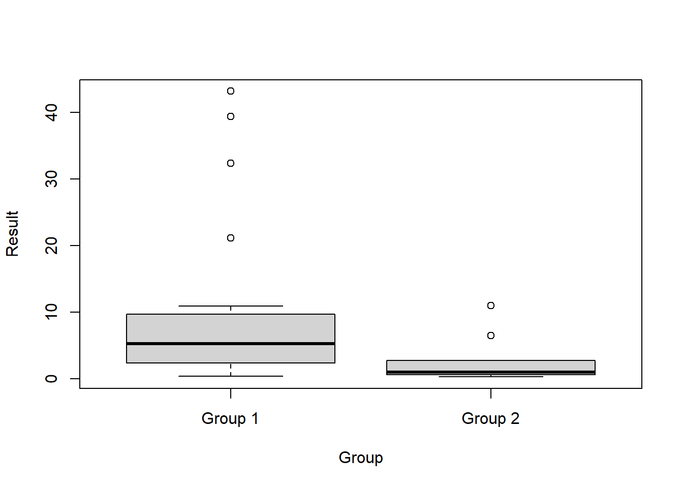
Descriptive statistics for each data set are shown below. The descriptive statistics include the total number of observations, detected observations, and frequency of detection; the minimum and maximum values for detected and non-detected observations; and the mean, median, standard deviation (SD), and coefficient of variation (CV) for each of the two groups. For this example, all observations are detects.
# Attach data
attach(dat)

# Get summary statistics using function
sumstats(dat, rv = 2, trans = TRUE)
##         Group 1 Group 2
## Obs       20.00   10.00
## Dets      20.00   10.00
## DetFreq  100.00  100.00
## MinND        NA      NA
## MinDET     0.37    0.26
## MaxND        NA      NA
## MaxDet    43.16   10.97
## Mean      10.45    2.57
## Median     5.21    0.95
## SD        12.97    3.48
## CV         1.24    1.35
Box plots comparing the two groups of data are provided below.
# Boxplots
boxplot(Result ~ Group, data = dat)
Wilcoxon Rank Sum Test
For comparison purposes, let’s test the null hypothesis that the mean of group 1 is equal to or less than the mean for group 2 against the alternative that the median for group 1 is greater than the median for group 2 using the WRS test.
wilcox.test(
  x = Result[Group == 'Group 1'],
  y = Result[Group == 'Group 2'],
  alternative = 'greater',
  mu = 0, paired = FALSE,
  conf.int = TRUE, conf.level = 0.95
)
##
## 	Wilcoxon rank sum exact test
##
## data:  Result[Group == "Group 1"] and Result[Group == "Group 2"]
## W = 158, p-value = 0.004808
## alternative hypothesis: true location shift is greater than 0
## 95 percent confidence interval:
##  1.309476      Inf
## sample estimates:
## difference in location
##               3.511922
The p-value for the WRS test is 0.005. Thus, at a typical significance level of 0.05, we reject the null hypothesis and accept the alternative that the median for group 1 is greater than the median for group 2.
Permutation Test: coin Package
The one-way() function in the coin package can be used to perform the Fisher-Pitman permutation test (Fisher 1936; Pitman 1937). The conditional null distribution of the test statistic is used to obtain p-values and an asymptotic approximation of the exact distribution is used by default (distribution = “symptotic”). Alternatively, the distribution can be approximated via Monte-Carlo resampling by setting the distribution variable to “approximate.”
# Load library
library(coin)

# Remove group ordering for coin package
dat2 <- dat %>%
  mutate(Group = factor(Group, ordered = FALSE))

# Run asymptotic Fisher-Pitman test
oneway_test(
  Result ~ Group, data = dat2,
  alternative = 'greater'
)
##
## 	Asymptotic Two-Sample Fisher-Pitman Permutation Test
##
## data:  Result by Group (Group 1, Group 2)
## Z = 1.796, p-value = 0.03624
## alternative hypothesis: true mu is greater than 0

# Run approximative (Monte Carlo) Fisher-Pitman test
set.seed(123)
oneway_test(
  Result ~ Group, data = dat2,
  distribution = approximate(nresample = 10000),
  alternative = 'greater'
)
##
## 	Approximative Two-Sample Fisher-Pitman Permutation Test
##
## data:  Result by Group (Group 1, Group 2)
## Z = 1.796, p-value = 0.0125
## alternative hypothesis: true mu is greater than 0
The p-values for the asymptotic approximation and the Monte-Carlo resampling are 0.036 and 0.013, respectively.
Permutation Test: EnvStats Package
The twoSamplePermutationTestLocation() function in the EnvStats package can be used to perform a two-sample or paired-sample permutation test for location based on either means or medians.
# Run test
perm_out <- twoSamplePermutationTestLocation(
  x = Result[Group == 'Group 1'],
  y = Result[Group == 'Group 2'],
  fcn = 'mean',
  alternative = 'greater',
  mu1.minus.mu2 = 0,
  paired = FALSE,
  exact = FALSE,
  n.permutations = 10000,
  seed = 123
)
print(perm_out)
##
## Results of Hypothesis Test
## --------------------------
##
## Null Hypothesis:                 mu.x-mu.y = 0
##
## Alternative Hypothesis:          True mu.x-mu.y is greater than 0
##
## Test Name:                       Two-Sample Permutation Test
##                                  Based on Differences in Means
##                                  (Based on Sampling
##                                  Permutation Distribution
##                                  10000 Times)
##
## Estimated Parameter(s):          mean of x = 10.449733
##                                  mean of y =  2.573186
##
## Data:                            x = Result[Group == "Group 1"]
##                                  y = Result[Group == "Group 2"]
##
## Sample Sizes:                    nx = 20
##                                  ny = 10
##
## Test Statistic:                  mean.x - mean.y = 7.876547
##
## P-value:                         0.0132
The p-value for the permutation test using the twoSamplePermutationTestLocation() function is 0.013.
Permutation Test: perm Package
The permTS() function in the perm package can be used to perform a two-sample permutation test. There is a choice of four different methods to calculate the p-value:
- pclt uses a permutational central limit theorem (Sen 1985)
- exact.mc uses Monte-Carlo simulation
- exact.network uses a network algorithm (Agresti et al. 1990)
- exact.ce uses complete enumeration for very small sample sizes
The variable permControl is used to create a list of arguments for controlling the permutation test. Let’s set the confidence level for the p-value estimate (p.conf.level) to 0.95, the number of Monte-Carlo replications (nmc) to 10,000, and the seed to 123.
# Load library
library(perm)

# Run test
permTS(
  x = Result[Group == 'Group 1'],
  y = Result[Group == 'Group 2'],
  method = 'exact.mc',
  alternative = 'greater',
  control = permControl(p.conf.level = 0.95, nmc = 10000, seed = 123)
)
##
## 	Exact Permutation Test Estimated by Monte Carlo
##
## data:  GROUP 1 and GROUP 2
## p-value = 0.011
## alternative hypothesis: true mean GROUP 1 - mean GROUP 2 is greater than 0
## sample estimates:
## mean GROUP 1 - mean GROUP 2
##                    7.876547
##
## p-value estimated from 10000 Monte Carlo replications
## 95 percent confidence interval on p-value:
##  0.008958341 0.013133833
The p-value for the permutation test using the permTS() function is 0.011.
Permutation Test: NADA2 Package
The cenperm2() function in the NADA2 package can be used to perform a two-sample permutation test for data with and without censored results.
# Load library
library(NADA2)

# Run permutation test
set.seed(123)
cenperm2(
  y1 = Result,
  y2 = Censored,
  grp = Group,
  R = 10000,
  alternative = 'greater',
  printstat = TRUE
)
##  Permutation test of mean CensData: Result   by Factor: Group
##      10000 Permutations     alternative = greater
##   mean of Group 1 = 10.45 to 10.45     mean of Group 2 = 2.573 to 2.573
##      Mean (Group 1 - Group 2) =  7.877 to 7.877       p = 0.0109989 to 0.0109989
##
The p-value for the permutation test using the cenperm2() function is 0.011.
Permutation Test: USGS Function
The perm2.R function included in Chapter 5 of Statistical Methods in Water Resources: U.S. Geological Survey Techniques and Methods, Book 4, Chapter A3 (Helsel et al. 2020) can be used to perform a permutation test for difference in the means associated with two groups of data. If the stacked variable is set to FALSE, the y1 and y2 variables are the two columns of data. Alternatively, if stacked is set to TRUE, the y1 variable represents the data and the y2 variable represents the groups.
I modified the perm2.R function, by adding a cc variable that let’s the user assign a reference factor for the two groups when setting stacked to TRUE. The default for cc is the first grouping factor.
Let’s first run the test using stacked set to FALSE.
# Load function
source('functions/perm2.R')

# Run test with stcaked set to FALSE
set.seed(123)
perm2(
  y1 = Result[Group == 'Group 1'],
  y2 = Result[Group == 'Group 2'],
  R = 10000,
  stacked = FALSE,
  alternative = 'g',
  conf = 0.95
)
##
##
##  Permutation Test of Difference Between 2 Group Means
## Data:  Result[Group == "Group 1"]  and  Result[Group == "Group 2"]
## Number of Possible Permutations is greater than 1000
##
##  R = 10000   pvalue = 0.0112
##  Alt Hyp: true difference in means is greater than 0
## sample estimates:
## mean of Result[Group == "Group 1"] = 10.44973    mean of Result[Group == "Group 2"] = 2.573186
## Diff of means = 7.876547
##      95 percent confidence interval
##            3.160836  Inf


Now, let’s run the test using stacked set to TRUE where y2 is the grouping variable. Let’s assign “Group 1” as the reference factor.
# Run test with stacked set to TRUE
set.seed(123)
perm2(
  y1 = Result,
  y2 = factor(Group, ordered = FALSE),
  cc = 'Group 1',
  R = 10000,
  stacked = TRUE,
  alternative = 'g',
  conf = 0.95
)
##
##
##  Permutation Test of Difference Between 2 Group Means
## Data:  Result  by  factor(Group, ordered = FALSE)
## Number of Possible Permutations is greater than 1000
##
##  R = 10000   pvalue = 0.0112
##  Alt Hyp: true difference in means is greater than 0
## sample estimates:
## mean of Group 1 = 10.44973    mean of Group 2 = 2.573186
## Diff of means = 7.876547
##      95 percent confidence interval
##            3.160836  Inf
The p-value for the permutation test using the perm2.R function is 0.011.
Conclusions
Permutation tests are designed to be robust against departures from normality. Permutation tests compute p-values by randomly selecting several thousand outcomes from the many larger number of outcomes possible that represent the null hypothesis. The p-value is then the proportion of outcomes that are equal to, or more extreme than, the one obtained from the actual data. When comparing central values of two independent groups of data, the two-sample t-test, the WRS test, or a two-sample permutation test might be selected. Test procedures should be selected based on the characteristics of the data and the objectives of interest. Of importance is whether the data have a particular distribution (such as a normal distribution) and if the central value under consideration is better defined by the mean (center of mass) or median (center of frequency). The advantage of a two-sample permutation test over a t-test is that there is no concern that a nonsignificant result might be a result that the input data substantially depart from the distributional assumption of the test.
References
Agresti, A., C.R. Mehta, and N.R. Patel. 1990. Exact Inference for Contingency Tables with Ordered Categories. JASA 85, 453-458.
Brown, D. and P. Rothery. 1993. Models in Biology: Mathematics, Statistics, and Computing. Wiley, New Jersey.
Good, P.I. 2005. Resampling Methods: A Practical Guide to Data Analysis. Third Edition. Birkhauser, Boston.
Helsel, D.R., R.M. Hirsch, K.R. Ryberg, S.A. Archfield, and E.J. Gilroy. 2020. Statistical Methods in Water Resources: U.S. Geological Survey Techniques and Methods, Book 4, Chapter A3. [Supersedes USGS Techniques of Water-Resources Investigations, Book 4, Chapter A3, Version 1.1.]. U.S. Geological Survey, Reston, Virginia.
Efron, B. and R.J. Tibshirani. 1993. An Introduction to the Bootstrap. Chapman and Hall, New York.
Fisher, R.A. 1936. The Coefficient of Racial Likeness and the Future of Craniometry. Journal of the Royal Anthropological Institute, 66, 57-63.
Manly, B.F.J. 2007. Randomization, Bootstrap and Monte Carlo Methods in Biology. Third Edition. Chapman & Hall, New York.
Millard, S.P. 2013. EnvStats: An R Package for Environmental Statistics. Springer-Verlag, NY.
Pitman, E.J.G. 1937. Significance Test Which May Be Applied to Samples From Any Populations. Supplement to the Journal of the Royal Statistical Society, 4, 119-130.
Sen, P.K. 1985. Permutational Central Limit Theorems. In S. Kotz and N.L. Johnson (eds.), Encyclopedia of Statistics, Volume 6. Wiley.
in Encyclopedia of Statistics, Vol 6.
- Posted on:
- December 22, 2022
- Length:
- 13 minute read, 2669 words
- See Also: