Clustering on Principal Component Analysis
By Charles Holbert
August 20, 2023
Introduction
Clustering is an important component of data analytics for discovering patterns in multivariate data sets. The goal is to identify groups (i.e., clusters) of similar objects within a data set of interest. Two common clustering methods are partitioning clustering, such as k-means clustering, and agglomerative hierarchical clustering. Partitioning clustering approaches subdivide the data sets into a set of k groups, where k is the number of groups pre-specified by the analyst. Hierarchical clustering does not require the analyst to pre-specify the number of clusters to be generated. The result is a tree-based representation of the objects, which is also known as dendrogram. Combining principal component analysis (PCA) and clustering methods are useful for reducing the dimension of the data into a few continuous variables containing the most important information in the data. Cluster analysis is then performed on the PCA results.
This post illustrates how to combine PCA and clustering methods using the R language for statistical computing and visualization.
Data
Let’s explore clustering of PCA using the Organisation for Economic Co-operation and Development (OECD) Better Life Index. The index describes the quality of life of a country’s inhabitants based on 11 topics, which are composed of one to three indicators. Within each topic, the indicators are averaged with equal weights. The indicators were chosen in consultation with OECD member countries on the basis of a number of statistical criteria, such as relevance and data quality. The objective of the index is to compare well-being across countries in the areas of material living conditions and quality of life. All data were taken from the OECD.
# Load libraries
library(dplyr)
library(clusterSim)
library(FactoMineR)
library(factoextra)
library(paran)
library(corrplot)

# Load data in comma-delimited file
datin <- read.csv('data/better_life_index_v2.csv', header = T)

# Remove columns that have missing values
dat <- datin %>%
  dplyr::select(where(~ !any(is.na(.))))

# Inspect structure of data
str(dat)
## 'data.frame':	32 obs. of  17 variables:
##  $ Country          : chr  "Australia" "Austria" "Belgium" "Canada" ...
##  $ employment.rate  : int  73 72 65 70 74 74 74 72 65 77 ...
##  $ unemployment.rate: num  1 1.3 2.3 0.5 0.6 0.9 1.2 1.2 2.9 1.2 ...
##  $ earnings         : int  55206 53132 54327 55342 29885 58430 30720 46230 45581 53745 ...
##  $ support.network  : int  93 92 90 93 96 95 95 96 94 90 ...
##  $ education.attain : int  84 86 80 92 94 82 91 91 81 86 ...
##  $ education.years  : int  20 17 19 17 18 19 18 20 17 18 ...
##  $ air.pollution    : num  6.7 12.2 12.8 7.1 17 10 5.9 5.5 11.4 12 ...
##  $ water.quality    : int  92 92 79 90 89 93 86 97 78 91 ...
##  $ regulation.engage: num  2.7 1.3 2 2.9 1.6 2 2.7 2.2 2.1 1.8 ...
##  $ voter.turnout    : int  92 76 88 68 62 85 64 69 75 76 ...
##  $ life.expectancy  : num  83 82 82.1 82.1 79.3 81.5 78.8 82.1 82.9 81.4 ...
##  $ health           : int  85 71 74 89 62 70 57 68 67 66 ...
##  $ life.satisfaction: num  7.1 7.2 6.8 7 6.9 7.5 6.5 7.9 6.7 7.3 ...
##  $ feeling.safe     : int  67 86 56 78 77 85 79 88 74 76 ...
##  $ homicide.rate    : num  0.9 0.5 1.1 1.2 0.7 0.5 1.9 1.2 0.4 0.4 ...
##  $ working.hours    : num  12.5 5.3 4.3 3.3 4.5 1.1 2.2 3.6 7.7 3.9 ...
Correlation Analysis
Although not definitive, including adjoining nearly correlated variables during PCA may increase the contribution of their common underlying factor to the PCA. Thus, there may be merit in discarding variables thought to be measuring the same underlying (but “latent”) aspect of a collection of variables before performing PCA.
Let’s explore correlations in our data.
# Get correlation matrix
cor.mat <- dat %>%
  dplyr::select(where(is.numeric)) %>%
  cor()

# Visualize the correlation matrix using corrplot
corrplot(
  cor.mat, type = 'lower', order = 'hclust',
  tl.col = 'black', tl.srt = 90
)
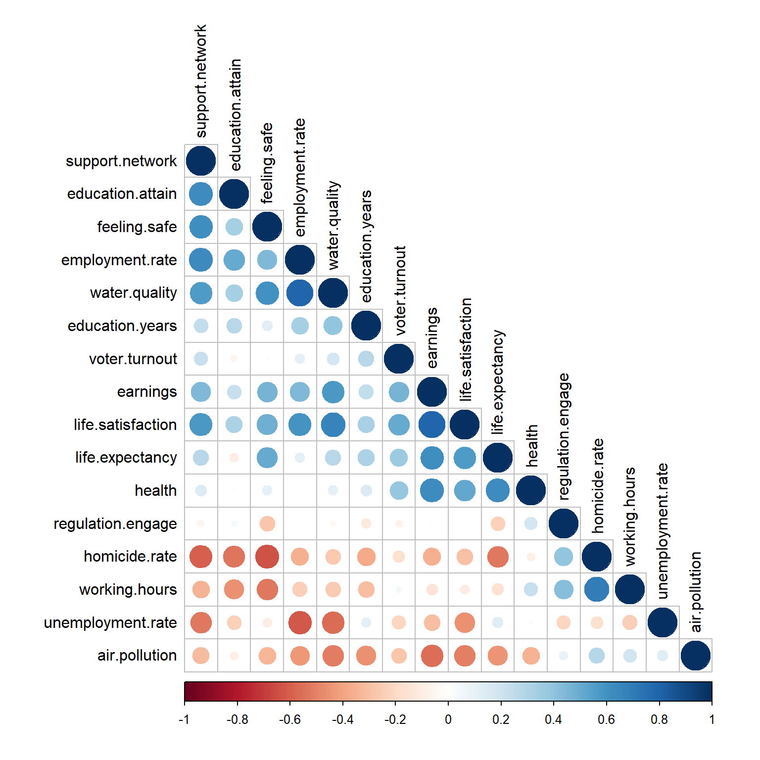
Now, let’s get a list of variables with an absolute value of the correlation coefficient greater than or equal to 0.8. A cut-off for highly correlated variables is often 0.8.
# Get variables with correlation coefficient greater than or equal to 0.8
cor.mat %>%
  data.frame() %>%
  mutate_if(is.numeric, round, 2) %>%
  tibble::rownames_to_column(var = 'rowname') %>%
  tidyr::gather(-rowname, key = "colname", value = "cor") %>%
  filter(abs(cor) >= 0.8) %>%
  mutate(flag = ifelse(rowname == colname, 1, 0)) %>%
  filter(flag == 0) %>%
  dplyr::select(-flag) %>%
  arrange(-cor, rowname)
##             rowname           colname cor
## 1          earnings life.satisfaction 0.8
## 2   employment.rate     water.quality 0.8
## 3 life.satisfaction          earnings 0.8
## 4     water.quality   employment.rate 0.8
Because PCA is a way to deal with highly correlated variables, let’s keep all the variables.
Multidimensional Scaling
Mathematically and conceptually, there are similarities between Multidimensional Scaling (MDS) and other methods used to reduce the dimensionality of complex data, such as PCA and factor analysis. While PCA is focused on the dimensions themselves, and seeks to maximize explained variance, MDS is more focused on relations among the scaled objects. MDS projects n-dimensional data points to a (commonly) 2-dimensional space such that similar objects in the n-dimensional space will be close together on the two dimensional plot. PCA projects a multidimensional space to the directions of maximum variability using covariance/correlation matrix to analyze the correlation between data points and variables.
Let’s perform MDS for all countries in our data. Distances between observations will be counted and then the distances in the 2-dimensional data will be optimized, so that they correspond to the distances in the original matrix. Finally, we will be inspect the MDS results to see if there are any clusters. Because the input variables have different scales of measurement, we will standardize the data prior to performing MDS or PCA. The data will be standardized by mean-centering and scaling to unit variance using the clusterSim package.
# Standardize data using clusterSim package
country <- dat[ ,1]
dat.norm <- data.Normalization(dat[, -1], type= 'n1', normalization = 'column')
rownames(dat.norm) <- country

# Perform MDS
mds <- dat.norm %>%
  dist() %>%
  cmdscale() %>%
  data.frame() %>%
  rename(Dim.1 = X1, Dim.2 = X2)

# Plot MDS
library(ggpubr)
ggscatter(
  mds, x = 'Dim.1', y = 'Dim.2',
  label = rownames(dat.norm),
  size = 1.5,
  font.label = c(10, 'plain'),
  repel = TRUE
) +
theme_bw()
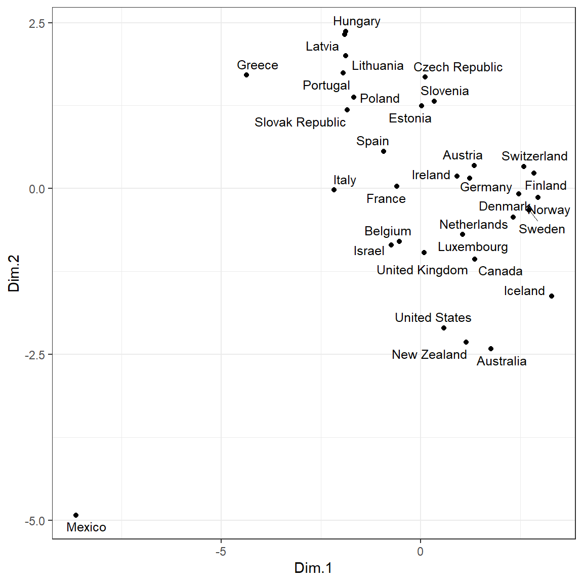
It appears that Mexico is far removed from the other countries and is an extreme outlier for these data. Let’s remove the outlier and rerun MDS.
# Remove outlier
dat <- dat[dat$Country != 'Mexico', ]
dat.norm <- dat.norm[rownames(dat.norm) != 'Mexico', ]

# Perform MDS
mds <- dat.norm %>%
  dist() %>%
  cmdscale() %>%
  data.frame() %>%
  rename(Dim.1 = X1, Dim.2 = X2)

# Plot MDS
library(ggpubr)
ggscatter(
  mds, x = 'Dim.1', y = 'Dim.2',
  label = rownames(dat.norm),
  size = 1.5,
  font.label = c(10, 'plain'),
  repel = TRUE
) +
theme_bw()
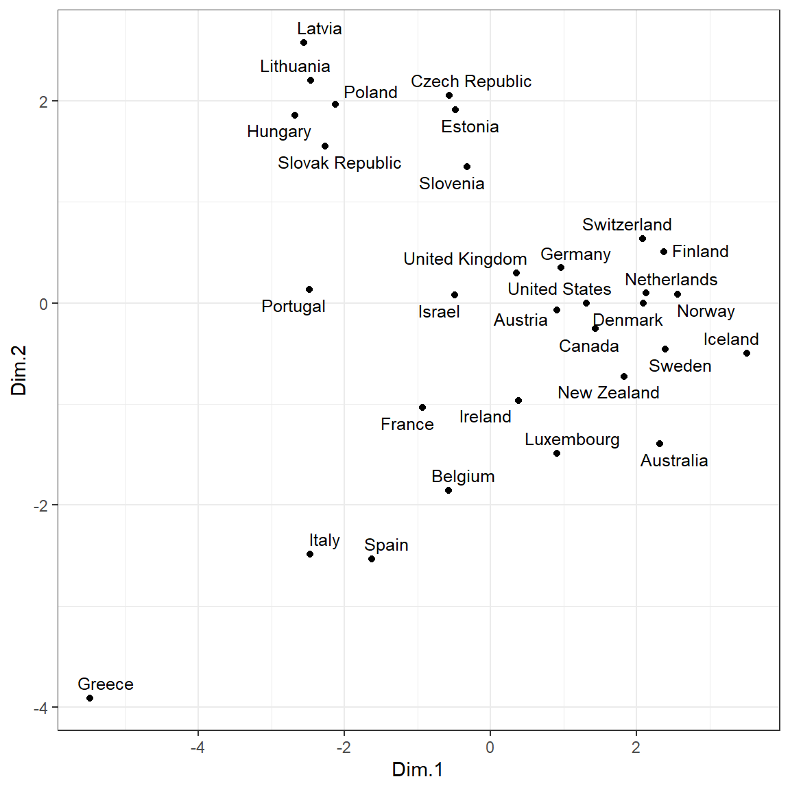
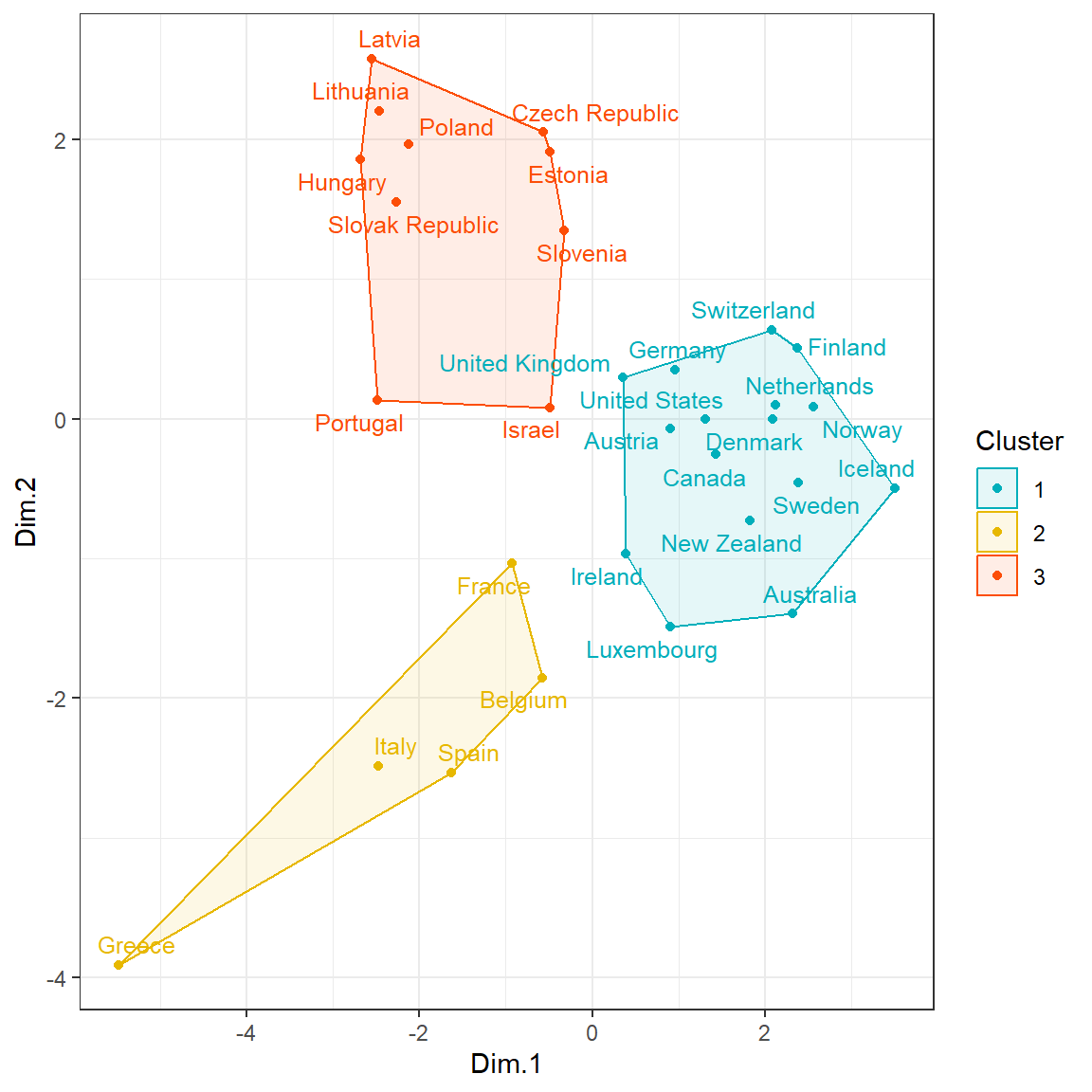
Let’s perform k-means clustering on the MDS results.
# K-means clustering on MDS
clust <- kmeans(mds, 3)$cluster %>%
  as.factor()
mds <- mds %>%
  mutate(Cluster = clust)

# Plot and color by groups
ggscatter(
  mds, x = 'Dim.1', y = 'Dim.2',
  label = rownames(dat.norm),
  color = 'Cluster',
  palette = c("#00AFBB", "#E7B800", "#FC4E07"),
  size = 1.5,
  font.label = c(10, 'plain'),
  show.legend.text = FALSE,
  ellipse = TRUE,
  ellipse.type = 'convex',
  repel = TRUE
) +
theme_bw()
Statistical Significance of PCA
Prior to conducting PCA, let’s evaluate the overall significance of PCA, of each principal component (PC) axis, and of the contributions of each variable to the significant axes based on permutation-based statistical tests. PCAtest uses random permutations to build null distributions for several statistics of a PCA analysis. Comparing these distributions with the observed values of the statistics, the function tests: (1) the hypothesis that there is more correlational structure among the observed variables than expected by random chance, (2) the statistical significance of each PC, and (3) the contribution of each observed variable to each significant PC.
# Load function
source('functions/PCAtest.R')

# Run PCA test on raw data because function centers and scales data
set.seed <- 1
result <- PCAtest(
  x = dat[, -1],
  nperm = 1000,
  nboot = 1000,
  alpha = 0.05,
  counter = FALSE,
  plot = TRUE
)
##
## ========================================================
## Test of PCA significance: 16 variables, 31 observations
## 1000 bootstrap replicates, 1000 random permutations
## ========================================================
##
## Empirical Psi = 26.1362, Max null Psi = 11.4210, Min null Psi = 5.0568, p-value = 0
## Empirical Phi = 0.3300, Max null Phi = 0.2181, Min null Phi = 0.1452, p-value = 0
##
## Empirical eigenvalue #1 = 5.01016, Max null eigenvalue = 3.37252, p-value = 0
## Empirical eigenvalue #2 = 2.83392, Max null eigenvalue = 2.59744, p-value = 0
## Empirical eigenvalue #3 = 1.94726, Max null eigenvalue = 2.25756, p-value = 0.158
## Empirical eigenvalue #4 = 1.41534, Max null eigenvalue = 1.93816, p-value = 0.983
## Empirical eigenvalue #5 = 1.11081, Max null eigenvalue = 1.70453, p-value = 1
## Empirical eigenvalue #6 = 0.81316, Max null eigenvalue = 1.49448, p-value = 1
## Empirical eigenvalue #7 = 0.75618, Max null eigenvalue = 1.40616, p-value = 1
## Empirical eigenvalue #8 = 0.53303, Max null eigenvalue = 1.12468, p-value = 1
## Empirical eigenvalue #9 = 0.44844, Max null eigenvalue = 1.01961, p-value = 1
## Empirical eigenvalue #10 = 0.35635, Max null eigenvalue = 0.85684, p-value = 1
## Empirical eigenvalue #11 = 0.23924, Max null eigenvalue = 0.72907, p-value = 1
## Empirical eigenvalue #12 = 0.19229, Max null eigenvalue = 0.64596, p-value = 1
## Empirical eigenvalue #13 = 0.13409, Max null eigenvalue = 0.52829, p-value = 1
## Empirical eigenvalue #14 = 0.1077, Max null eigenvalue = 0.41776, p-value = 1
## Empirical eigenvalue #15 = 0.06422, Max null eigenvalue = 0.31461, p-value = 0.999
## Empirical eigenvalue #16 = 0.03783, Max null eigenvalue = 0.23417, p-value = 0.993
##
## PC 1 is significant and accounts for 31.3% (95%-CI:26.9-39.7) of the total variation
## PC 2 is significant and accounts for 17.7% (95%-CI:15.4-23.9) of the total variation
##
## The first 2 PC axes are significant and account for 49% of the total variation
##
## Variables 1, 2, 3, 4, 7, 8, 12, 13, and 14 have significant loadings on PC 1
## Variables 5, and 11 have significant loadings on PC 2
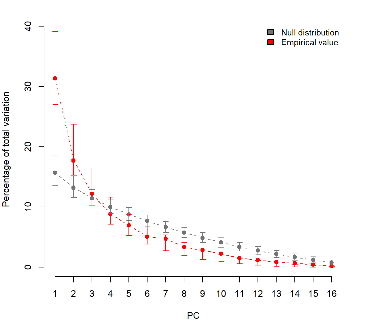
The results from PCAtest indicates that the first 2 PCs are significant.
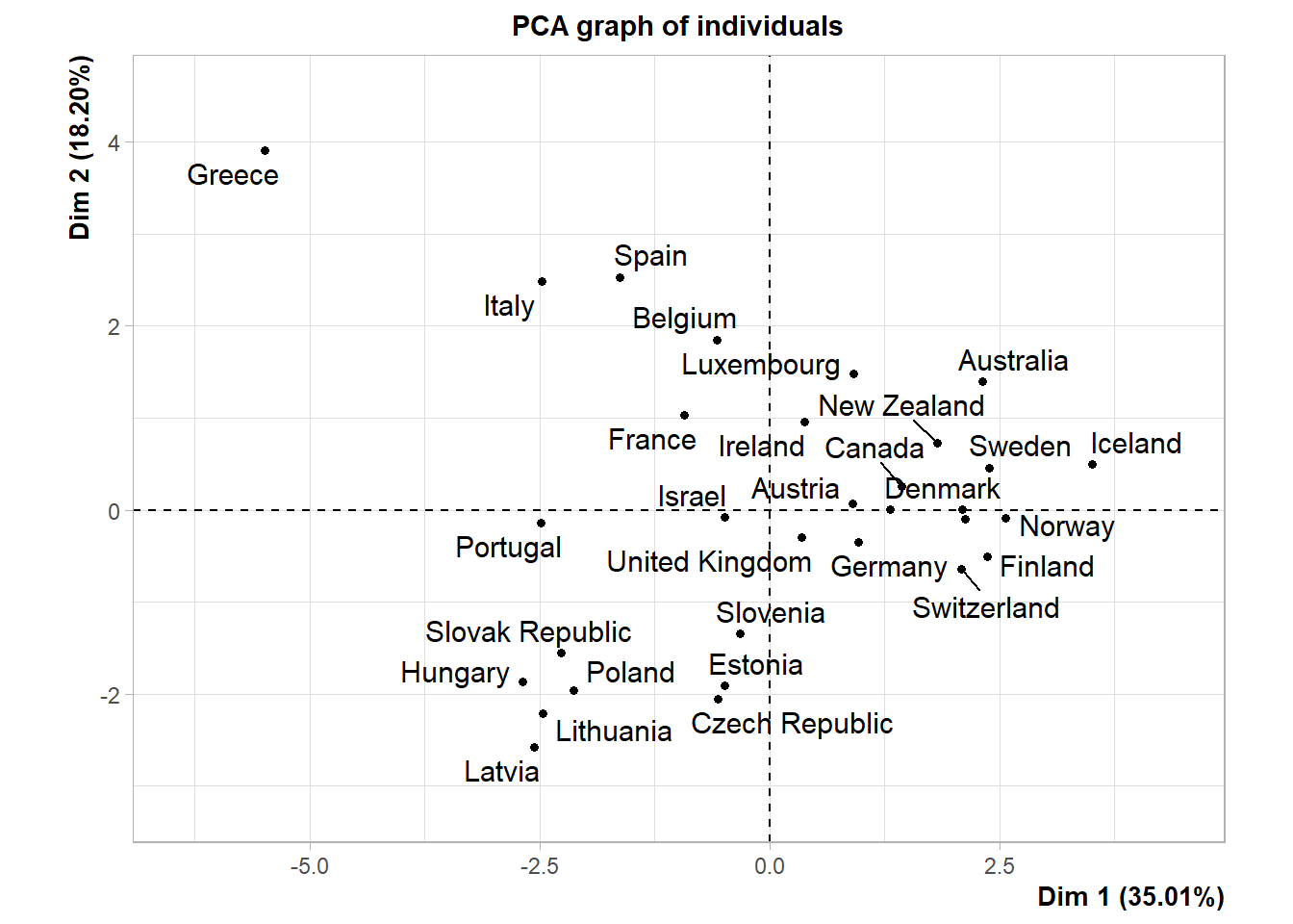
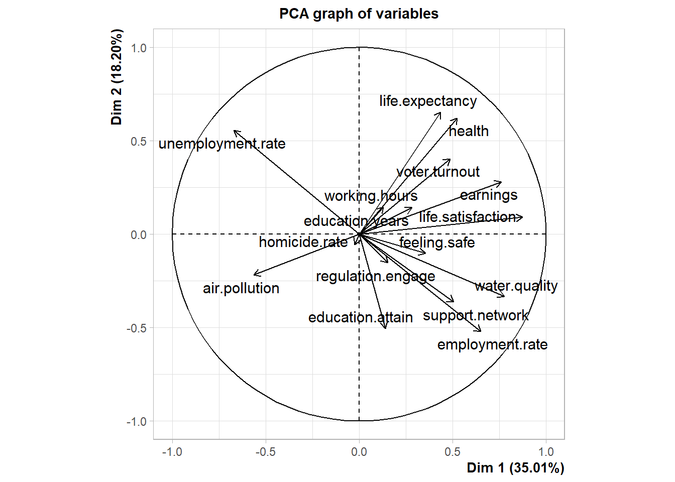
Principal Component Analysis
Let’s perform PCA on the normalized data using the PCA() function in the FactoMineR package.
# Perform PCA
dat.pca <- PCA(
  dat.norm,
  scale.unit = FALSE,
  ind.sup = NULL,
  quali.sup = NULL,
  graph = TRUE
)

# Add the coordinates to the data
dat.norm <- cbind(dat.norm, dat.pca$ind$coord)
Let’s review a summary of the PCA results.
# Summary of PCA results
summary(dat.pca)
##
## Call:
## PCA(X = dat.norm, scale.unit = FALSE, ind.sup = NULL, quali.sup = NULL,
##      graph = TRUE)
##
##
## Eigenvalues
##                        Dim.1   Dim.2   Dim.3   Dim.4   Dim.5   Dim.6   Dim.7
## Variance               4.366   2.270   1.333   1.081   0.881   0.563   0.462
## % of var.             35.009  18.203  10.688   8.670   7.068   4.512   3.705
## Cumulative % of var.  35.009  53.212  63.900  72.571  79.638  84.151  87.856
##                        Dim.8   Dim.9  Dim.10  Dim.11  Dim.12  Dim.13  Dim.14
## Variance               0.430   0.300   0.200   0.191   0.163   0.108   0.059
## % of var.              3.448   2.405   1.603   1.529   1.309   0.870   0.475
## Cumulative % of var.  91.304  93.709  95.313  96.841  98.150  99.020  99.494
##                       Dim.15  Dim.16
## Variance               0.052   0.011
## % of var.              0.417   0.089
## Cumulative % of var.  99.911 100.000
##
## Individuals (the 10 first)
##                       Dist    Dim.1    ctr   cos2    Dim.2    ctr   cos2
## Australia         |  3.801 |  2.316  3.962  0.371 |  1.396  2.770  0.135 |
## Austria           |  2.343 |  0.907  0.608  0.150 |  0.069  0.007  0.001 |
## Belgium           |  3.254 | -0.577  0.246  0.031 |  1.852  4.873  0.324 |
## Canada            |  2.743 |  1.434  1.519  0.273 |  0.256  0.093  0.009 |
## Czech Republic    |  2.763 | -0.563  0.234  0.041 | -2.055  6.002  0.553 |
## Denmark           |  2.673 |  2.092  3.233  0.613 |  0.002  0.000  0.000 |
## Estonia           |  2.771 | -0.484  0.173  0.031 | -1.911  5.189  0.476 |
## Finland           |  3.433 |  2.369  4.148  0.476 | -0.509  0.368  0.022 |
## France            |  2.001 | -0.929  0.638  0.216 |  1.036  1.524  0.268 |
## Germany           |  2.013 |  0.964  0.686  0.229 | -0.349  0.173  0.030 |
##                    Dim.3    ctr   cos2
## Australia          1.185  3.396  0.097 |
## Austria           -1.106  2.962  0.223 |
## Belgium            0.650  1.023  0.040 |
## Canada             1.295  4.060  0.223 |
## Czech Republic    -0.507  0.622  0.034 |
## Denmark           -0.953  2.199  0.127 |
## Estonia           -0.151  0.055  0.003 |
## Finland           -1.188  3.416  0.120 |
## France             0.463  0.519  0.054 |
## Germany           -0.790  1.512  0.154 |
##
## Variables (the 10 first)
##                      Dim.1    ctr   cos2    Dim.2    ctr   cos2    Dim.3    ctr
## employment.rate   |  0.651  9.717  0.483 | -0.521 11.942  0.308 | -0.141  1.487
## unemployment.rate | -0.670 10.275  0.460 |  0.556 13.613  0.317 | -0.177  2.338
## earnings          |  0.761 13.264  0.667 |  0.280  3.462  0.091 |  0.072  0.386
## support.network   |  0.505  5.847  0.408 | -0.363  5.808  0.211 |  0.146  1.606
## education.attain  |  0.142  0.460  0.032 | -0.505 11.224  0.412 |  0.303  6.902
## education.years   |  0.282  1.823  0.093 |  0.142  0.884  0.023 | -0.236  4.167
## air.pollution     | -0.565  7.304  0.358 | -0.218  2.100  0.054 |  0.258  4.980
## water.quality     |  0.776 13.799  0.645 | -0.334  4.919  0.120 | -0.325  7.912
## regulation.engage |  0.154  0.540  0.026 | -0.153  1.034  0.026 |  0.690 35.692
## voter.turnout     |  0.487  5.431  0.240 |  0.404  7.176  0.165 |  0.129  1.240
##                     cos2
## employment.rate    0.023 |
## unemployment.rate  0.032 |
## earnings           0.006 |
## support.network    0.034 |
## education.attain   0.149 |
## education.years    0.065 |
## air.pollution      0.075 |
## water.quality      0.113 |
## regulation.engage  0.531 |
## voter.turnout      0.017 |
The cumulative variance of the first two PCs is equal to 53.2%. This is lower than we would like and thus, more than two PCs may be needed to adequately explain the variance in the data. To determine an optimal number of PCs, two methods will be used: the Kaiser criterion and adjusting the scree plot results with parallel analysis.
Kaiser Criterion
The Kaiser criterion helps to establish an optimal number of PCs that adequately explains the variance in the data. According to the criterion, the number of PCs should equal the number of eigenvalues with values greater than one.
# Table of eigenvalues
get_eigenvalue(dat.pca)
##        eigenvalue variance.percent cumulative.variance.percent
## Dim.1  4.36605234      35.00901711                    35.00902
## Dim.2  2.27018552      18.20339234                    53.21241
## Dim.3  1.33290665      10.68785895                    63.90027
## Dim.4  1.08130115       8.67037030                    72.57064
## Dim.5  0.88142360       7.06766010                    79.63830
## Dim.6  0.56275121       4.51239821                    84.15070
## Dim.7  0.46208942       3.70524565                    87.85594
## Dim.8  0.43006250       3.44843905                    91.30438
## Dim.9  0.29992934       2.40497150                    93.70935
## Dim.10 0.19994432       1.60324561                    95.31260
## Dim.11 0.19065112       1.52872846                    96.84133
## Dim.12 0.16318597       1.30850023                    98.14983
## Dim.13 0.10846218       0.86969970                    99.01953
## Dim.14 0.05918630       0.47458300                    99.49411
## Dim.15 0.05202683       0.41717504                    99.91129
## Dim.16 0.01106381       0.08871474                   100.00000
There are four eigenvalues with values greater than 1; therefore, according to the criterion, four PCs should be chosen.
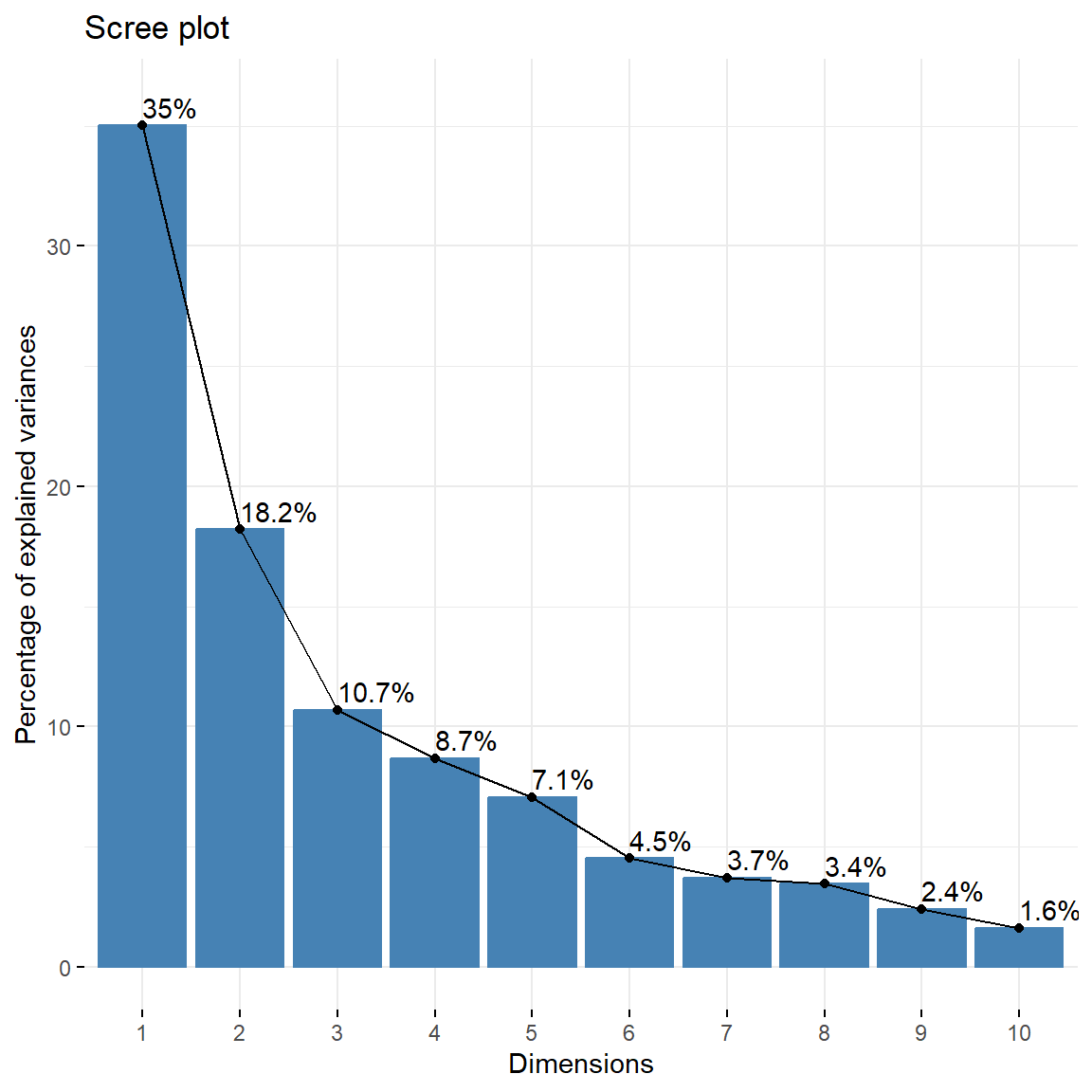
Scree Plot
An alternative method to determine the number of PCs is to look at a scree plot, which is the plot of eigenvalues ordered from largest to the smallest for each PC. A scree plot displays how much variation each PC captures from the data. The number of components is determined at the point, beyond which the remaining eigenvalues are all relatively small and of comparable size.
# Create Scree plot using factoextra
fviz_eig(dat.pca, addlabels = TRUE, ylim = c(0, 36))
Parallel analysis with scree plot was introduced by Horn (1965). Parallel analysis is an empirical method designed to both graphically and numerically assess the number of components to keep in PCA. It is based on the assumption that if data are random, non-correlated factors would be observed and eigenvalues of PCA would be equal to one. Horn’s technique compares actual PCA results with the random data PCA results.
Let’s use the paran package to perform Horn’s parallel analysis.
# Perform Horn's parallel analysis for PCA
paran(
  dat.norm,
  iterations = 10000, quietly = FALSE,
  status = FALSE, all = TRUE, cfa = FALSE, graph = TRUE,
  color = TRUE, col = c('black', 'red', 'blue'),
  lty = c(1, 2, 3), lwd = 1, legend = TRUE, file = "",
  width = 1200, height = 1200, grdevice = 'png',
  seed = 0, mat = NA, n = NA
)
##
## Using eigendecomposition of correlation matrix.
##
## Results of Horn's Parallel Analysis for component retention
## 10000 iterations, using the mean estimate
##
## --------------------------------------------------
## Component   Adjusted    Unadjusted    Estimated
##             Eigenvalue  Eigenvalue    Bias
## --------------------------------------------------
## 1           4.139064    6.008731      1.869667
## 2           2.358415    3.817785      1.459370
## 3           1.733958    2.893740      1.159781
## 4           1.474455    2.388383      0.913928
## 5           1.342919    2.043849      0.700930
## 6           0.410012    0.919454      0.509441
## 7           0.451284    0.789347      0.338063
## 8           0.362484    0.543050      0.180566
## 9           0.416555    0.454733      0.038177
## 10          0.455557    0.362155     -0.09340
## 11          0.455377    0.240318     -0.21505
## 12          0.519364    0.192746     -0.32661
## 13          0.562361    0.134250     -0.42811
## 14          0.631220    0.108552     -0.52266
## 15          0.671518    0.064623     -0.60689
## 16          0.721793    0.038275     -0.68351
## 17          0.752019    0.000000     -0.75201
## 18          0.812300    0.000000     -0.81230
## 19          0.865714    0.000000     -0.86571
## 20          0.911629   0.000000     -0.91162
## 21          0.951992   0.000000     -0.95199
## --------------------------------------------------
##
## Adjusted eigenvalues > 1 indicate dimensions to retain.
## (5 components retained)

The graph can be evaluated in two ways:
- Retain factors which have adjusted eigenvalue higher than one
- Retain factors which real PCA eigenvalues are higher than randomly generated ones
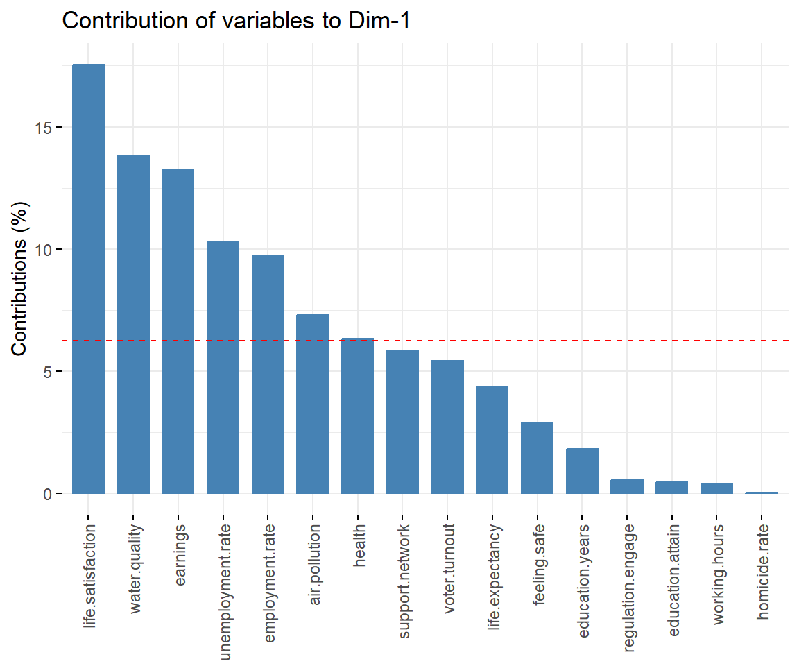
Contributions
Let’s see which variables contribute the most for the first four PCs.
View contributions of variables to PC 1.
# Contributions of variables to PC1
fviz_contrib(dat.pca, 'var', axes = 1, xtickslab.rt = 90)
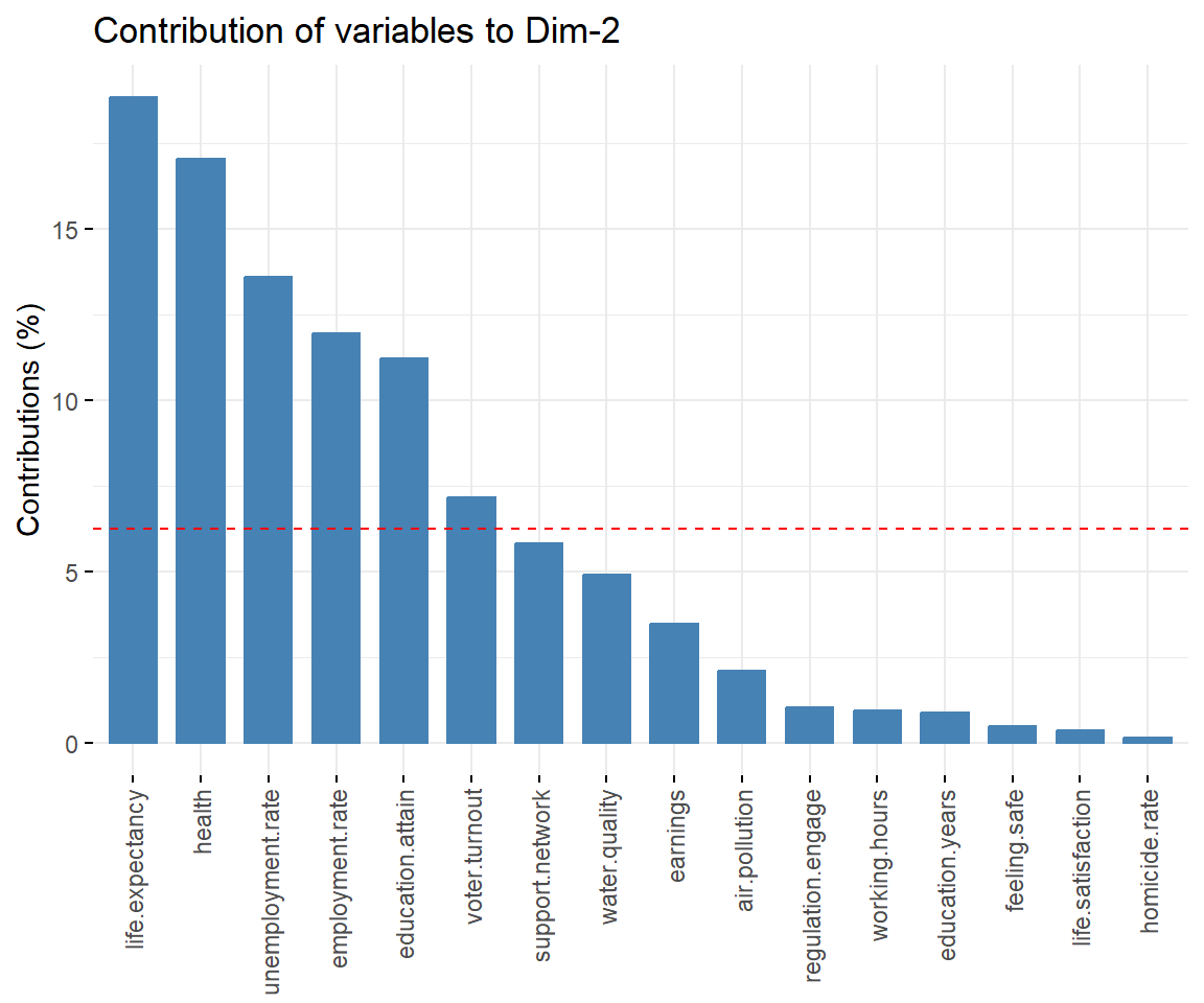
View contributions of variables to PC 2.
# Contributions of variables to PC2
fviz_contrib(dat.pca, 'var', axes = 2, xtickslab.rt = 90)
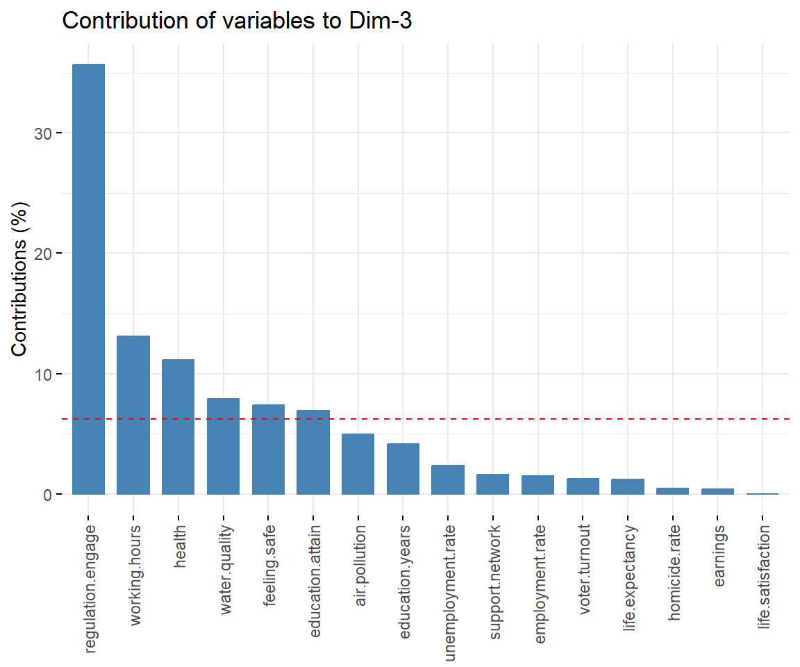
View contributions of variables to PC 3.
# Contributions of variables to PC3
fviz_contrib(dat.pca, 'var', axes = 3, xtickslab.rt = 90)
View contributions of variables to PC 4.
# Contributions of variables to PC4
fviz_contrib(dat.pca, 'var', axes = 4, xtickslab.rt = 90)
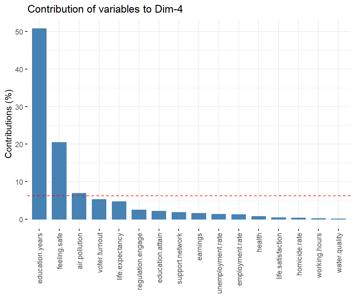
Let’s get tabulated output showing which variables are the most correlated to the first four PCs.
dimdesc(
  PCA(
    dat.norm,
    scale.unit = FALSE,
    ind.sup = NULL,
    quali.sup = NULL,
    graph = FALSE
  ),
  axes = 1:4
)
## $Dim.1
##
## Link between the variable and the continuous variables (R-square)
## =================================================================================
##                   correlation      p.value
## Dim.1               1.0000000 0.000000e+00
## life.satisfaction   0.9100867 1.290541e-12
## earnings            0.8166796 2.110028e-08
## water.quality       0.8033139 5.339010e-08
## employment.rate     0.6947807 1.446140e-05
## support.network     0.6389774 1.092989e-04
## health              0.5267119 2.333895e-03
## voter.turnout       0.4898950 5.150913e-03
## life.expectancy     0.4826858 5.955545e-03
## feeling.safe        0.4476301 1.156782e-02
## air.pollution      -0.5986879 3.736911e-04
## unemployment.rate  -0.6779041 2.789440e-05
##
## $Dim.2
##
## Link between the variable and the continuous variables (R-square)
## =================================================================================
##                   correlation      p.value
## Dim.2               1.0000000 0.000000e+00
## life.expectancy     0.7222829 4.487281e-06
## health              0.6239350 1.764325e-04
## unemployment.rate   0.5626411 9.850459e-04
## voter.turnout       0.4060498 2.341912e-02
## support.network    -0.4592419 9.353466e-03
## employment.rate    -0.5553976 1.181331e-03
## education.attain   -0.6419171 9.923870e-05
##
## $Dim.3
##
## Link between the variable and the continuous variables (R-square)
## =================================================================================
##                   correlation       p.value
## Dim.3               1.0000000 1.550177e-228
## regulation.engage   0.7287920  3.333604e-06
## working.hours       0.5831303  5.756988e-04
## health              0.3858149  3.206257e-02
## education.attain    0.3857054  3.211553e-02
## feeling.safe       -0.3956796  2.757205e-02
##
## $Dim.4
##
## Link between the variable and the continuous variables (R-square)
## =================================================================================
##                 correlation      p.value
## Dim.4             1.0000000 0.000000e+00
## education.years   0.8014945 6.025323e-08
## feeling.safe     -0.5919489 4.518349e-04
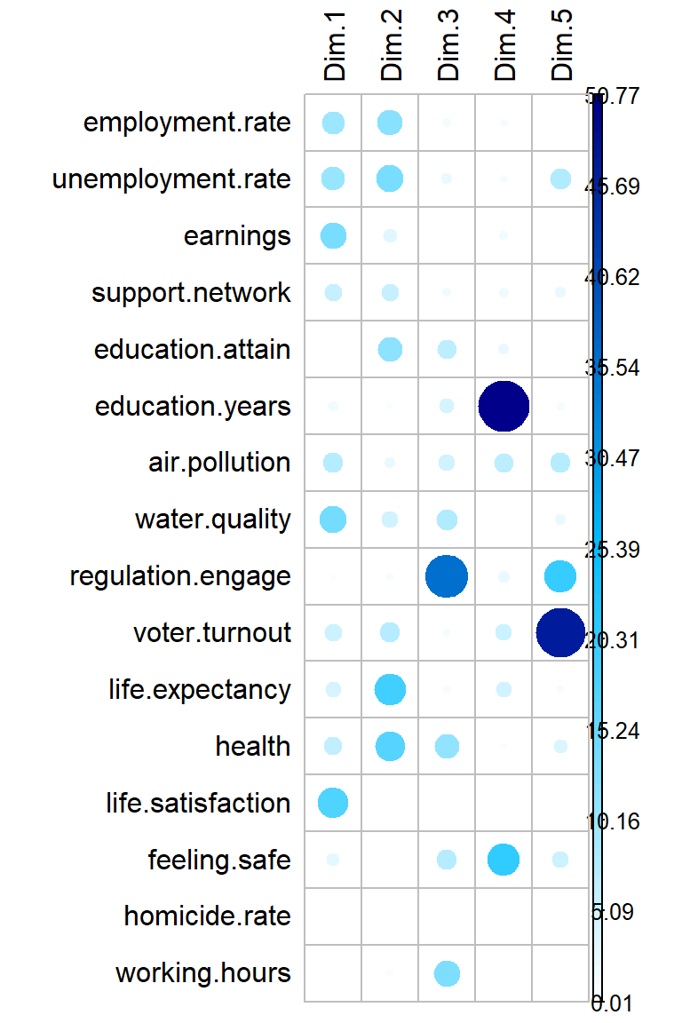
Let’s highlight variables contributing the most information for each dimension.
corrplot(
  dat.pca$var$contrib, is.corr = FALSE,
  tl.col = 'black',
  col = colorRampPalette(c('white', 'deepskyblue', 'blue4'))(100)
)
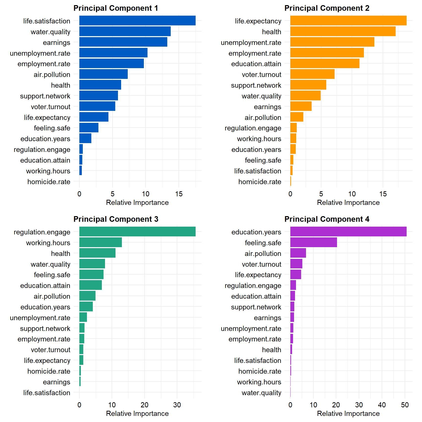
Relative Importance Plots
Let’s create plots showing the relative importance of the variables to each of the first four PCs.
# Get contributions for each PC
tidied_pca <- bind_cols(
  Parameter = rownames(dat.pca$var$contrib),
  data.frame(dat.pca$var$contrib)
  ) %>%
  rename(PC1 = Dim.1, PC2 = Dim.2, PC3 = Dim.3, PC4 = Dim.4, PC5 = Dim.5) %>%
  tidyr::gather(PC, Contribution, PC1:PC5)

# Create list of plotting elements
gglayer_theme <- list(
  theme_minimal(),
  theme(
    plot.title = element_text(margin = margin(b = 3), size = 12, hjust = 0,
                              color = 'black', face = 'bold'),
    plot.margin = unit(c(0.1, 0.2, 0.1, 0.2), 'in'),
    axis.title.y = element_text(size = 11, color = 'black'),
    axis.title.x = element_text(size = 11, color = 'black'),
    axis.text.x = element_text(size = 11, color = 'black'),
    axis.text.y = element_text(size = 11, color = 'black')
  )
)

# Create plot for PC1
p1 <- tidied_pca %>%
  filter(PC == 'PC1') %>%
  mutate(Parameter = reorder(Parameter, Contribution)) %>%
  ggplot(aes(x = Contribution, y = Parameter)) +
  geom_col(show.legend = FALSE, fill = '#005BC3') +
  labs(title = 'Principal Component 1',
       x = 'Relative Importance',
       y = NULL) +
  gglayer_theme

# Create plot for PC2
p2 <- tidied_pca %>%
  filter(PC == 'PC2') %>%
  mutate(Parameter = reorder(Parameter, Contribution)) %>%
  ggplot(aes(x = Contribution, y = Parameter)) +
  geom_col(show.legend = FALSE, fill = '#FF9A00') +
  labs(title = 'Principal Component 2',
       x = 'Relative Importance',
       y = NULL) +
  gglayer_theme

# Create plot for PC3
p3 <- tidied_pca %>%
  filter(PC == 'PC3') %>%
  mutate(Parameter = reorder(Parameter, Contribution)) %>%
  ggplot(aes(x = Contribution, y = Parameter)) +
  geom_col(show.legend = FALSE, fill = '#21A582') +
  labs(title = 'Principal Component 3',
       x = 'Relative Importance',
       y = NULL) +
  gglayer_theme

# Create plot for PC4
p4 <- tidied_pca %>%
  filter(PC == 'PC4') %>%
  mutate(Parameter = reorder(Parameter, Contribution)) %>%
  ggplot(aes(x = Contribution, y = Parameter)) +
  geom_col(show.legend = FALSE, fill = '#AA2ED0') +
  labs(title = 'Principal Component 4',
       x = 'Relative Importance',
       y = NULL) +
  gglayer_theme

# Put all plots together
cowplot::plot_grid(
  p1, p2, p3, p4,
  nrow = 2
)
Clustering Assessment
Before applying any clustering algorithm to a data set, the first thing to do is to assess the clustering tendency (are the data suitable for clustering). If the data are suitable for clustering, the next step is to determine an optimal number of clusters. Once this is done, hierarchical clustering or partitioning clustering (with a pre-specified number of clusters) can be performed.
Clustering Tendency
Both hierarchical and k-means clustering can impose a classification on a random uniformly distributed data set even if the data contain no meaningful clusters. The Hopkins statistic is used to assess the clustering tendency of a data set by measuring the probability that a given data set is generated by a uniform data distribution. In other words, it tests the spatial randomness of the data. If the value of Hopkins statistic is near 0.5, the data are uniformly distributed. If the value of the Hopkins statistic is far from 0.5, the data are clusterable.
Let’s evaluate the clustering tendency for our data using the get_clust_tendency() function from the factoextra package.
res <- get_clust_tendency(dat.norm, n = nrow(dat.norm)-1, graph = FALSE)
res$hopkins
## [1] 0.6273689
The Hopkins statistic is 0.63, which is not very optimistic concerning the clusterable of the data. However, let’s see if performing PCA before clustering will give better results.
Number of Clusters
Determining the optimal number of clusters in a data set is a fundamental issue in partitioning clustering, such as k-means clustering. The optimal number of clusters can be subjective and generally depends on the method used for measuring similarities and the parameters used for partitioning. Two commonly used methods are the silhouette method and the gap statistic. In addition to these two methods, there are more than thirty other indices and methods that have been published for identifying the optimal number of clusters.
The silhouette method computes the average silhouette of observations for different values of k. The optimal number of clusters k is the one that maximize the average silhouette over a range of possible values for k (Kaufman and Rousseeuw 1990). The gap statistic (Tibshirani et al. 2001) compares the total within intra-cluster variation for different values of k with their expected values under the null reference distribution of the data. The estimate of the optimal clusters will be the value that maximizes the gap statistic (i.e, that yields the largest gap statistic). Thus, the basic idea of the gap statistic is to choose the k, where the biggest jump in within-cluster distance occurs.
Let’s apply both methods to our data.
# Computes average silhouette of observations for different values of k
fviz_nbclust(
  dat.pca$ind$coord,
  FUNcluster = kmeans,
  method = 'silhouette', k.max = 8
)

## Get gap statistic
fviz_nbclust(
  dat.pca$ind$coord,
  FUNcluster = kmeans,
  method = 'gap_stat', k.max = 8
) +
theme_classic()
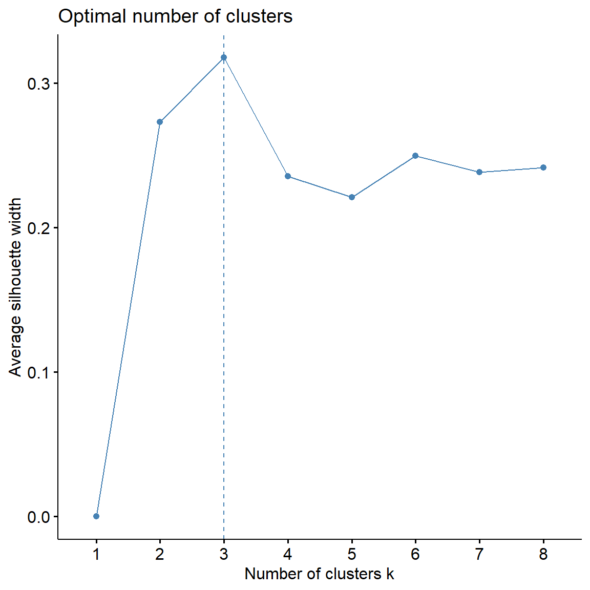
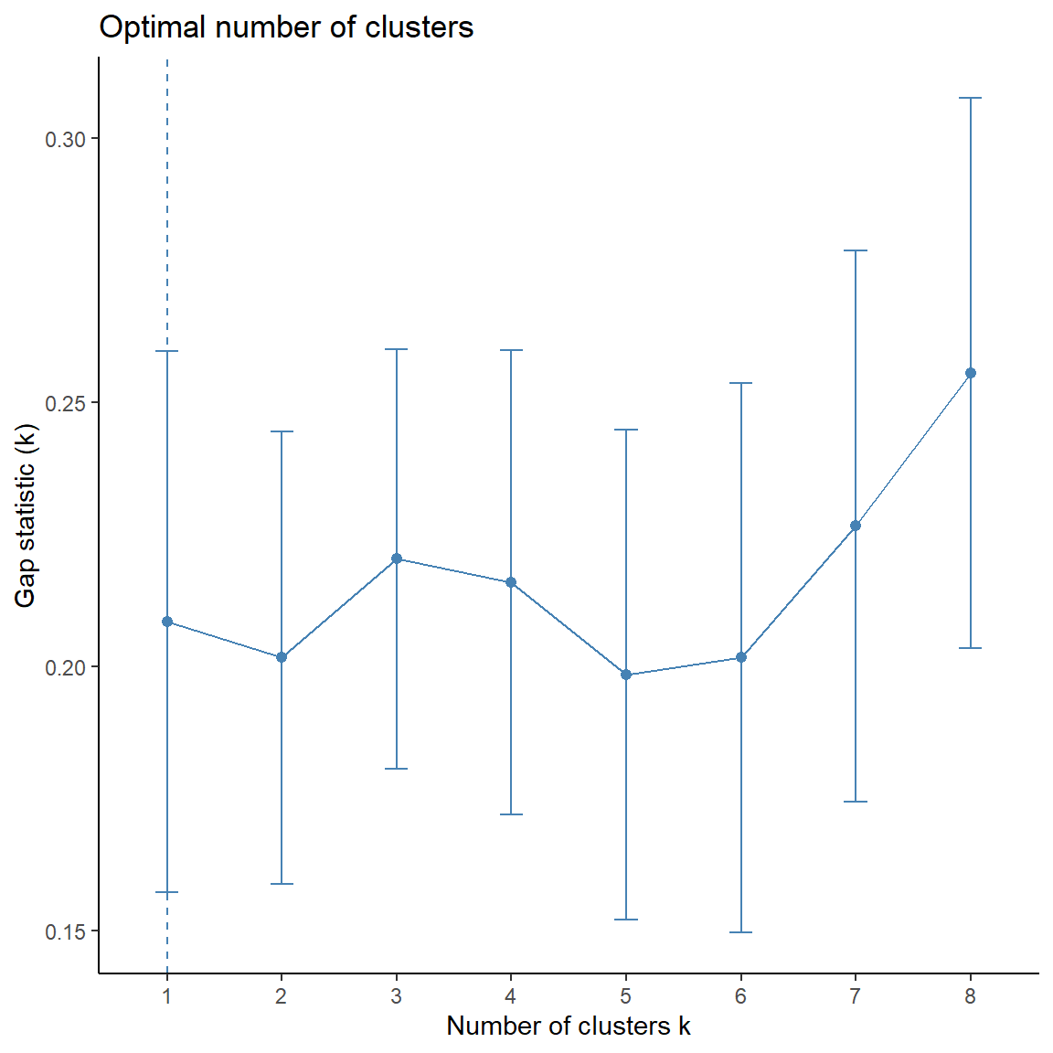
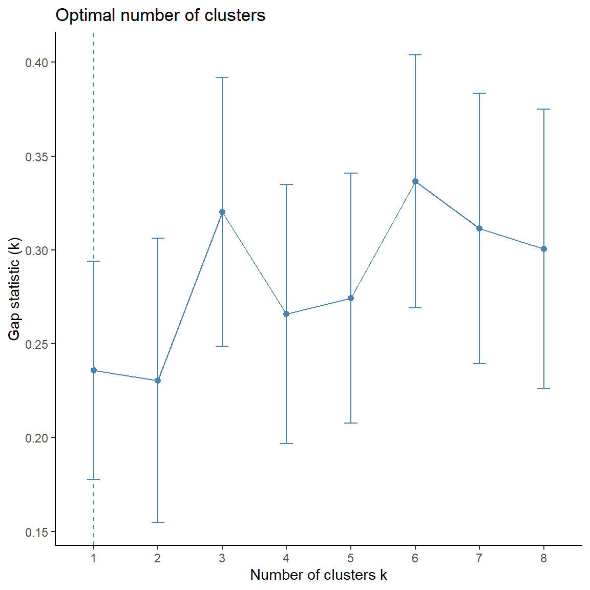
The silhouette statistic is the highest for 3 clusters. The biggest differences for the gap statistic are visible for 1 and 3 clusters.
The NbClust] package provides 30 indices for determining the relevant number of clusters and proposes to users the best clustering scheme from the different results obtained by varying all combinations of number of clusters, distance measures, and clustering methods. It simultaneously computes all indices and determines the number of clusters in a single function call.
# Finding the relevant number of clusters using NbClust package
library(NbClust)
NbClust(
  dat.pca$ind$coord, distance = 'euclidean',
  min.nc = 2, max.nc = 8,
  method = 'complete', index = 'alllong'
)
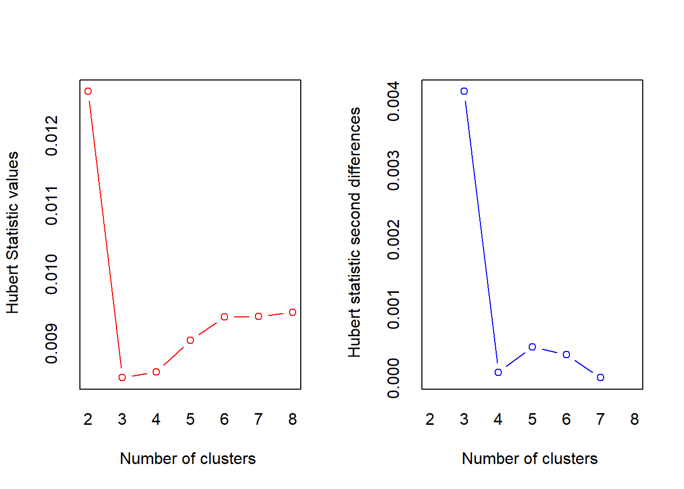
## *** : The Hubert index is a graphical method of determining the number of clusters.
##                 In the plot of Hubert index, we seek a significant knee that corresponds to a
##                 significant increase of the value of the measure i.e the significant peak in Hubert
##                 index second differences plot.
##
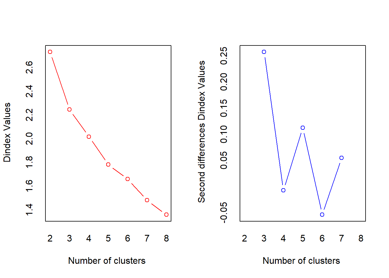
## *** : The D index is a graphical method of determining the number of clusters.
##                 In the plot of D index, we seek a significant knee (the significant peak in Dindex
##                 second differences plot) that corresponds to a significant increase of the value of
##                 the measure.
##
## *******************************************************************
## * Among all indices:
## * 12 proposed 2 as the best number of clusters
## * 10 proposed 3 as the best number of clusters
## * 2 proposed 5 as the best number of clusters
## * 3 proposed 7 as the best number of clusters
## * 1 proposed 8 as the best number of clusters
##
##                    ***** Conclusion *****
##
## * According to the majority rule, the best number of clusters is  2
##
##
## *******************************************************************
## $All.index
##       KL      CH Hartigan     CCC    Scott   Marriot    TrCovW   TraceW
## 2 0.4467  5.7879  13.8172 -3.5768  28.4196 576507749 3270.8044 256.6628
## 3 4.3263 10.7958   5.3857 -1.9765  75.8967 280451307 1521.6081 173.8370
## 4 0.4006 10.0062   8.0032 -2.2714  99.5972 232114746  979.3835 145.7940
## 5 2.3429 11.2955   4.3747 -1.1762 152.9978  64774953  530.9060 112.4594
## 6 0.6620 10.9921   5.5652 -1.1783 174.9857  45891227  413.5158  96.2623
## 7 2.1221 11.6417   3.2354 -0.4111 206.8627  22337952  291.9068  78.7354
## 8 0.9971 11.2949   3.0927 -0.5477 232.0265  12956706  245.8692  69.3820
##   Friedman  Rubin Cindex     DB Silhouette   Duda Pseudot2   Beale Ratkowsky
## 2   0.8860 1.1996 0.5016 0.4020     0.4769 0.6773  13.3408  1.4398    0.2195
## 3   5.0428 1.7711 0.4563 1.0741     0.3012 0.7257   6.4242  1.1170    0.2514
## 4   7.6321 2.1118 0.5033 1.2302     0.2136 0.5343   7.8432  2.4548    0.2745
## 5  14.8695 2.7378 0.4586 1.1226     0.2557 0.7264   3.7659  1.0715    0.2834
## 6  16.7015 3.1984 0.4695 1.1070     0.2721 0.5071   6.8039  2.6619    0.2921
## 7  21.5825 3.9104 0.4704 0.9578     0.2972 0.9570   0.0449  0.0703    0.2983
## 8  27.6884 4.4376 0.4597 0.8275     0.3277 1.0448  -0.2144 -0.1118    0.2866
##       Ball Ptbiserial     Gap   Frey McClain  Gamma   Gplus     Tau   Dunn
## 2 128.3314     0.5747 -0.7683 3.7368  0.0356 0.9390  0.8559 26.3527 0.5975
## 3  57.9457     0.5716 -1.0213 3.0713  0.6806 0.6840 18.3548 79.4495 0.3564
## 4  36.4485     0.4459 -1.4933 0.0050  1.5277 0.5738 21.0215 56.5935 0.2213
## 5  22.4919     0.5053 -1.6481 0.3558  1.7820 0.7155 12.5247 63.0065 0.2310
## 6  16.0437     0.4965 -1.8354 0.2920  2.3349 0.7721  8.3419 56.5075 0.2598
## 7  11.2479     0.4844 -2.0722 0.0940  2.9348 0.8231  5.3204 49.5183 0.2887
## 8   8.6728     0.4869 -2.0799 0.2488  2.9867 0.8373  4.7806 49.2000 0.2895
##   Hubert SDindex Dindex   SDbw
## 2 0.0126  0.6250 2.7281 0.4132
## 3 0.0085  0.9219 2.2435 0.3815
## 4 0.0086  1.1916 2.0159 0.3331
## 5 0.0090  1.1361 1.7810 0.2833
## 6 0.0094  1.0981 1.6583 0.2781
## 7 0.0094  1.0869 1.4816 0.2381
## 8 0.0094  0.9877 1.3593 0.1657
##
## $All.CriticalValues
##   CritValue_Duda CritValue_PseudoT2 Fvalue_Beale CritValue_Gap
## 2         0.5344            24.3907       0.2137        0.2792
## 3         0.4477            20.9744       0.3575        0.5112
## 4         0.3141            19.6526       0.0475        0.2081
## 5         0.3379            19.5956       0.3874        0.2478
## 6         0.2552            20.4342       0.0385        0.3033
## 7        -0.1969            -6.0787       0.9944        0.0809
## 8         0.1725            23.9899       1.0000        0.5101
##
## $Best.nc
##                     KL      CH Hartigan     CCC   Scott   Marriot   TrCovW
## Number_clusters 3.0000  7.0000   3.0000  7.0000  5.0000         3    3.000
## Value_Index     4.3263 11.6417   8.4315 -0.4111 53.4006 247719881 1749.196
##                  TraceW Friedman   Rubin Cindex    DB Silhouette   Duda
## Number_clusters  3.0000   5.0000  3.0000 3.0000 2.000     2.0000 2.0000
## Value_Index     54.7828   7.2374 -0.2309 0.4563 0.402     0.4769 0.6773
##                 PseudoT2  Beale Ratkowsky    Ball PtBiserial     Gap   Frey
## Number_clusters   2.0000 2.0000    7.0000  3.0000     2.0000  2.0000 3.0000
## Value_Index      13.3408 1.4398    0.2983 70.3857     0.5747 -0.7683 3.0713
##                 McClain Gamma  Gplus     Tau   Dunn Hubert SDindex Dindex
## Number_clusters  2.0000 2.000 2.0000  3.0000 2.0000      0   2.000      0
## Value_Index      0.0356 0.939 0.8559 79.4495 0.5975      0   0.625      0
##                   SDbw
## Number_clusters 8.0000
## Value_Index     0.1657
##
## $Best.partition
##       Australia         Austria         Belgium          Canada  Czech Republic
##               1               1               1               1               1
##         Denmark         Estonia         Finland          France         Germany
##               1               1               1               1               1
##          Greece         Hungary         Iceland         Ireland          Israel
##               2               1               1               1               1
##           Italy          Latvia       Lithuania      Luxembourg     Netherlands
##               1               1               1               1               1
##     New Zealand          Norway          Poland        Portugal Slovak Republic
##               1               1               1               1               1
##        Slovenia           Spain          Sweden     Switzerland  United Kingdom
##               1               1               1               1               1
##   United States
##               1
There are 12 methods in the NbClust] package that proposed 2 clusters while 10 methods proposed 3 clusters. According to the majority rule, the best number of clusters is 2.
The Optimal_Clusters_KMeans() function of the ClusterR package can be used to determined the optimal number of clusters for the k-means algorithm.
# Finding the relevant number of clusters using ClusterR
library(ClusterR)
Optimal_Clusters_KMeans(
  dat.pca$ind$coord,
  max_clusters = 8,
  criterion = 'distortion_fK',
  fK_threshold = 0.85,
  num_init = 1,
  max_iters = 200,
  initializer = 'kmeans++',
  tol = 1e-04,
  plot_clusters = TRUE,
  verbose = FALSE,
  tol_optimal_init = 0.3,
  seed = 1,
  mini_batch_params = NULL
)
## [1] 1.0000000 0.8025031 1.0738679 0.8149165 0.9090035 1.1479858 0.9047884
## [8] 0.8625168
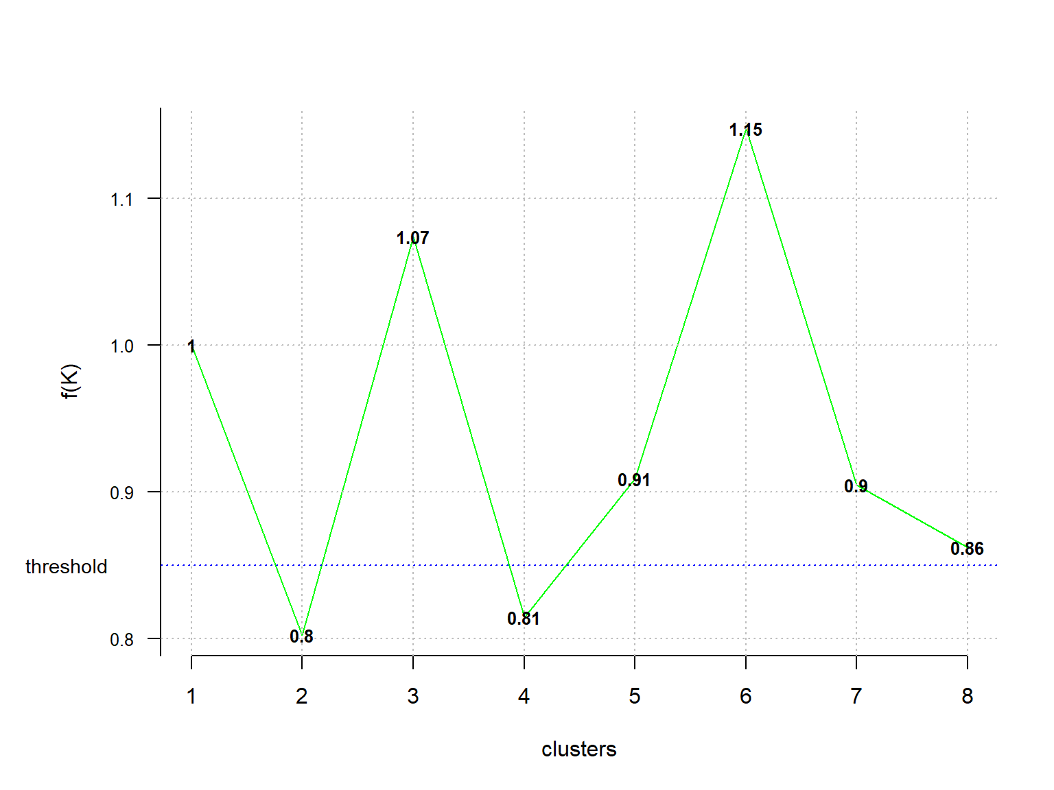
Values below the fixed threshold (here fK_threshold = 0.85) are recommended for clustering. For our data there are multiple optimal clusters (2 and 4). When this occurs, the final decision as to which value to use is left to the discretion of the analyst.
K-Means Clustering on PCs
The next step is to choose the most suitable distance metric. For that purpose, clustering for the following two different distance measures will be conducted: (1) Euclidean distance and (2) Manhattan distance. For most clustering software, the default distance measure is Euclidean distance where observations with high values of features will be clustered together. Manhattan distance places less emphasis on outlying observations. First, let’s rerun PCA where the number of PCs will be set to 2.
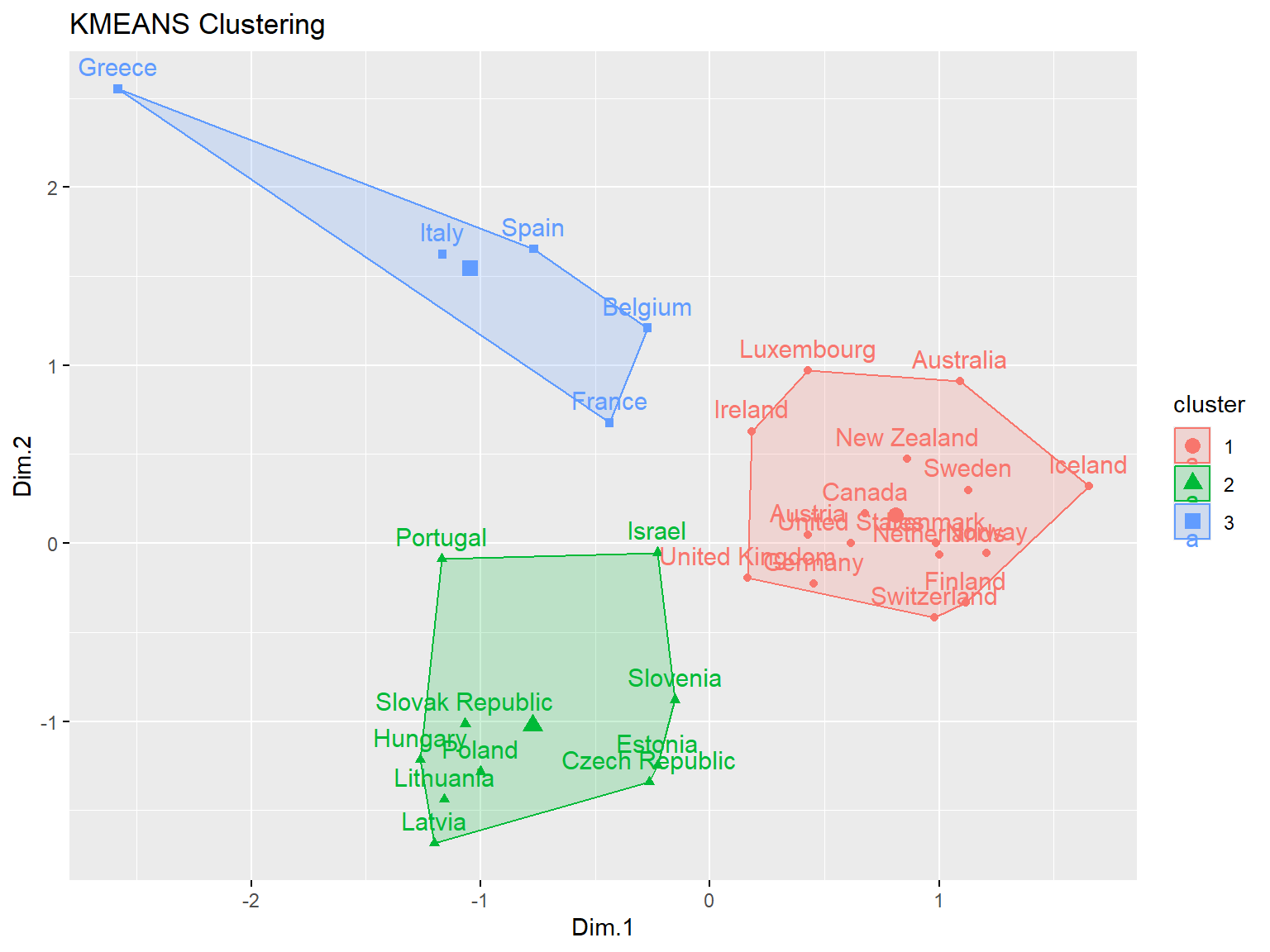
Let’s conduct k-means clustering on PCA results using Euclidean distance.
# PCA with number of PCs set to 2.
dat.pca <- PCA(
dat.norm,
scale.unit = FALSE,
ncp = 2,
ind.sup = NULL,
quali.sup = NULL,
graph = FALSE
)
# Add coordinates to the data
dat.norm$Dim.1 <- NULL
dat.norm$Dim.2 <- NULL
dat.norm$Dim.3 <- NULL
dat.norm$Dim.4 <- NULL
dat.norm$Dim.5 <- NULL
dat.norm <- cbind(dat.norm, dat.pca$ind$coord)
# Euclidean distance
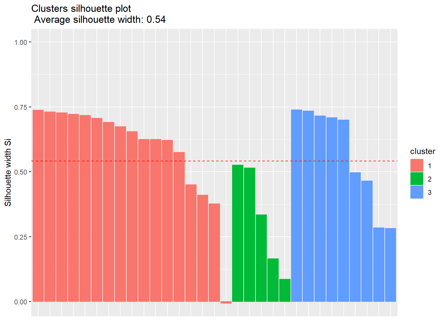
km1 <- eclust(dat.pca$ind$coord, 'kmeans', hc_metric = 'eucliden', k = 3)
fviz_silhouette(km1)
## cluster size ave.sil.width
## 1 1 16 0.63
## 2 2 10 0.50
## 3 3 5 0.33

Now, let’s conduct k-means clustering on PCA results using Manhattan distance.
# Manhattan distance
km2 <- eclust(dat.pca$ind$coord, 'kmeans', hc_metric = 'manhattan', k = 3)
fviz_silhouette(km2)
##   cluster size ave.sil.width
## 1       1   16          0.63
## 2       2   10          0.50
## 3       3    5          0.33

Both measures have the same silhouette statistic, hence there is no difference in distances. The average silhouette is equal to 0.54, which means that clustering quality is not ideal.
PAM Clustering on PCs
The second method of clustering is Partitioning Around Medoids (PAM) algorithm, which is a more robust version of k-means clustering and less sensitive to outliers. The overall goal PAM clustering is to cluster points around medoids instead of artificial points as is done in k-means clustering.
As before, let’s establish the optimal number of clusters.
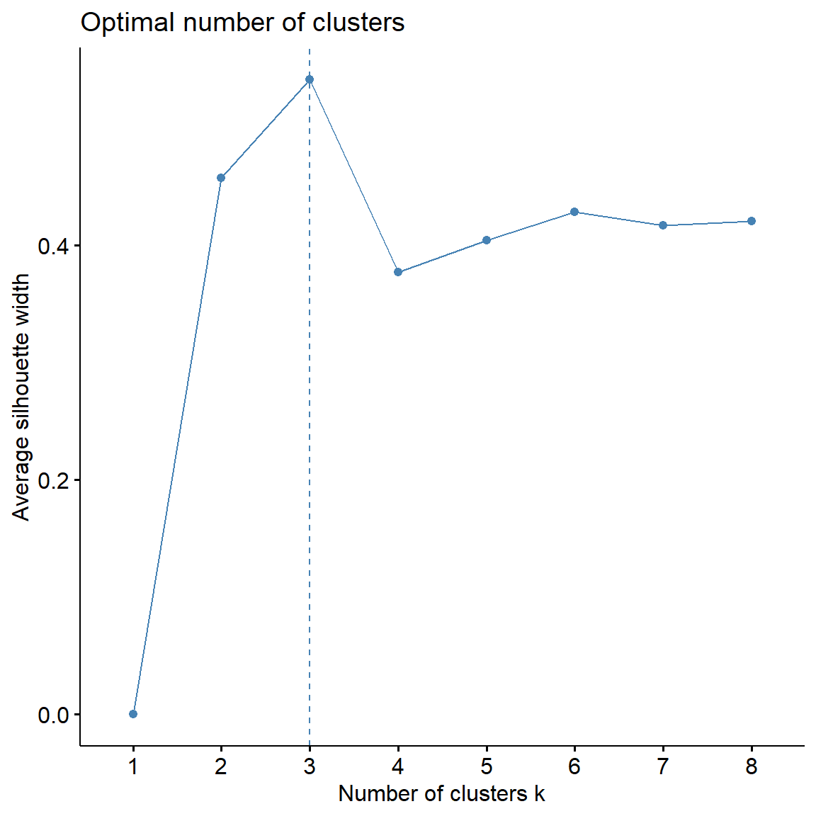
# Computes average silhouette of observations for different values of k
fviz_nbclust(
  dat.pca$ind$coord,
  FUNcluster = cluster::pam,
  method = 'silhouette', k.max = 8
)

## Get gap statistic
fviz_nbclust(
  dat.pca$ind$coord,
  FUNcluster = cluster::pam,
  method = 'gap_stat', k.max = 8
) +
theme_classic()
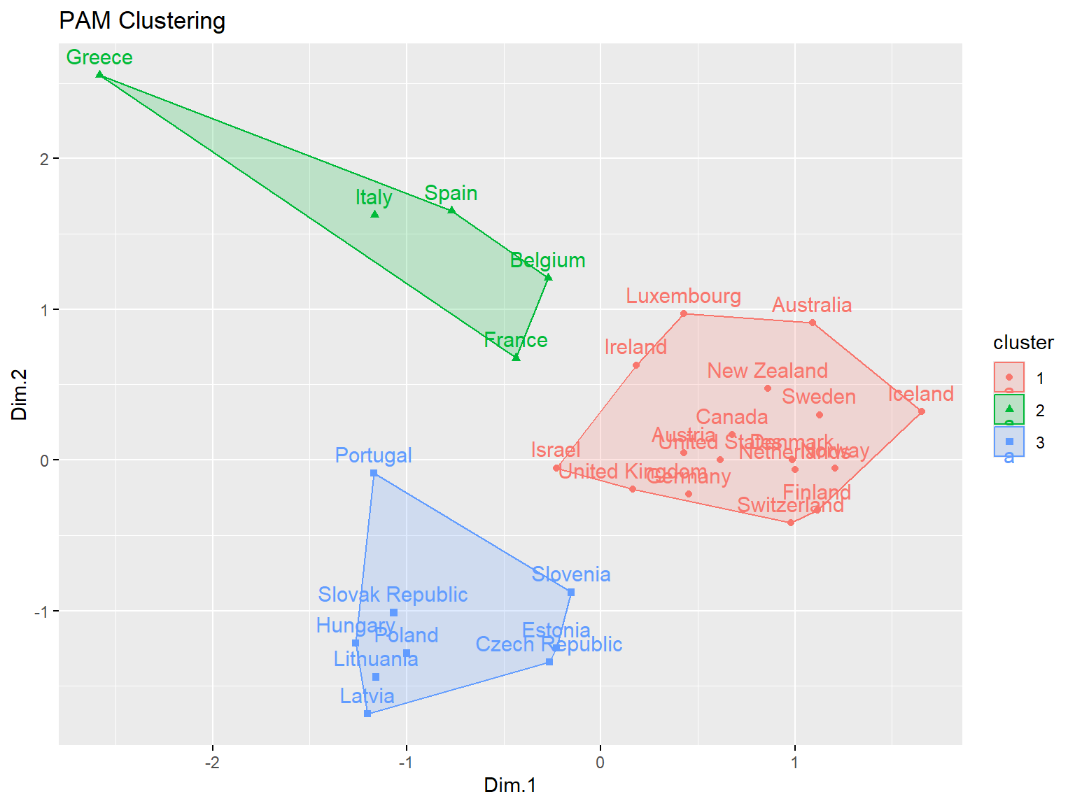
Now, let’s perform PAM clustering using 3 clusters.
# Clustering with PAM
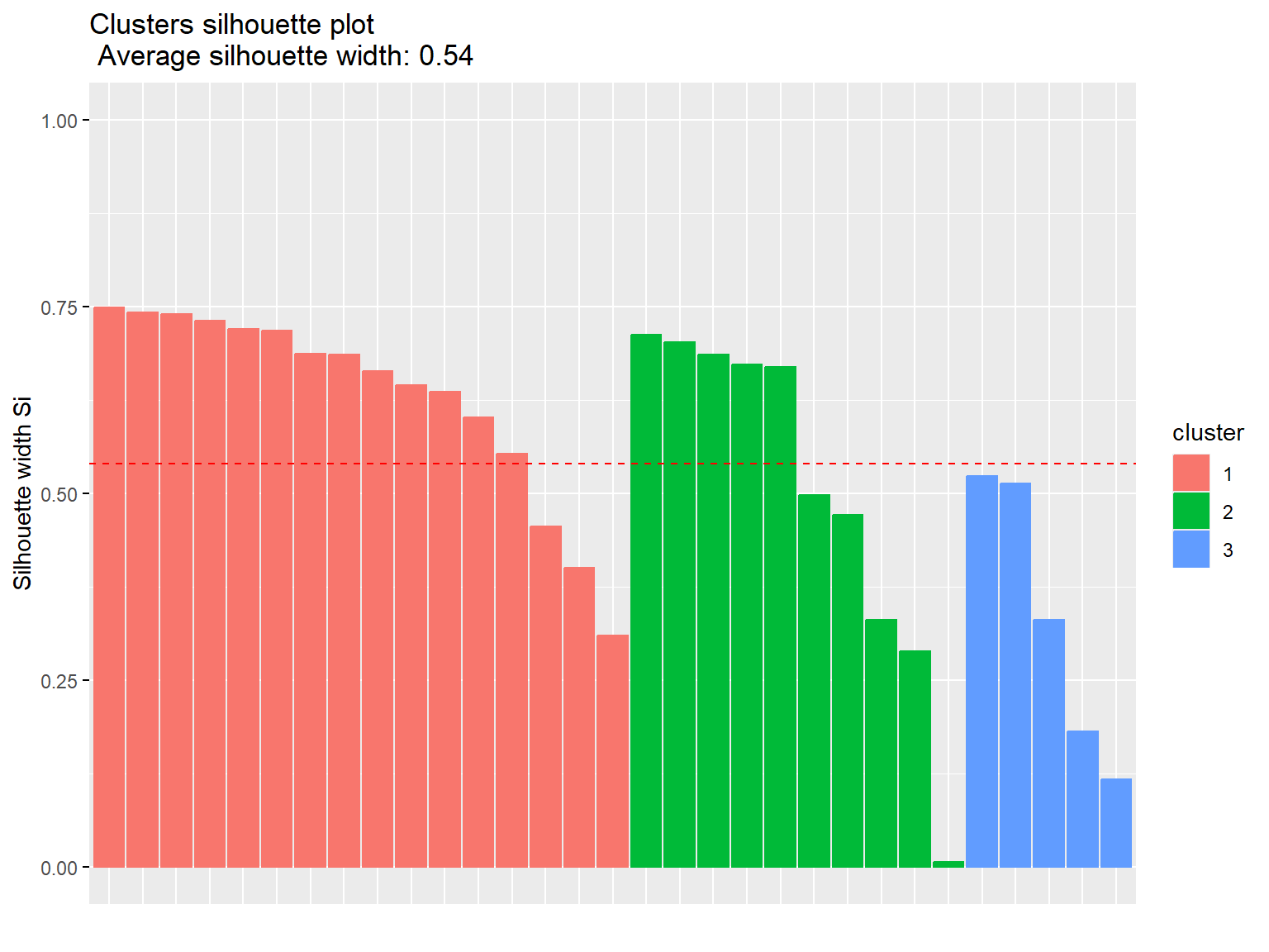
pm <- eclust(dat.pca$ind$coord, 'pam', k = 3)
fviz_silhouette(pm)
## cluster size ave.sil.width
## 1 1 17 0.59
## 2 2 5 0.33
## 3 3 9 0.57
The results obtained using PAM clustering are the same as those obtained with k-means clustering.
Hierarchical Clustering on PCs
Hierarchical clustering on principal components (HCPC) is an unsupervised method, meaning that no information about class membership is required prior to the analysis. This makes HCPC suitable for exploratory data analysis, where the aim is hypothesis generation rather than hypothesis verification. The goal of the clustering algorithm is to partition objects into homogeneous groups, such that the within-group similarities are large compared to the between-group similarities. The result is a dendrogram, which presents the hierarchy of the clusters.
Let’s perform hierarchical clustering on the PCs from our PCA where the number of PCs was set to 2
# Compute hierarchical clustering on principal components
dat.hcpc <- HCPC(dat.pca, graph = F)

# Add clusters to data
dat.norm$clust <- dat.hcpc$data.clust$clust
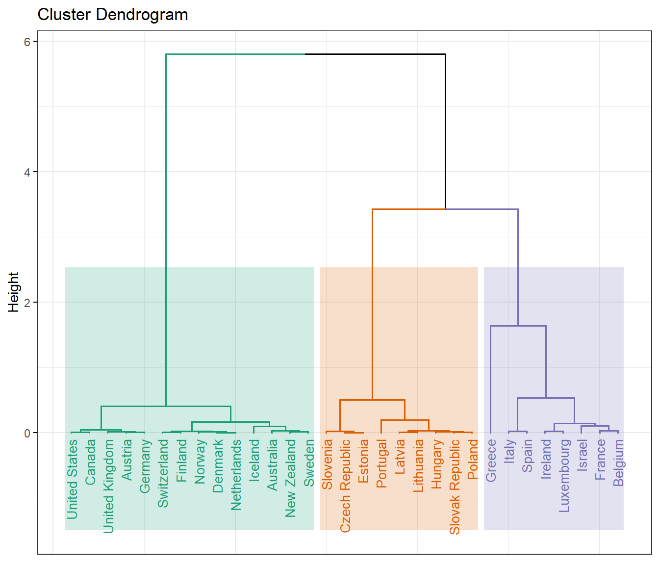
Let’s create the dendrogram based on the HCPC. The distance of split or merge (called height) is shown on the y-axis of the dendrogram.
# Create dendrogram
fviz_dend(
  dat.hcpc,
  ggtheme = theme_bw(),
  cex = 0.7, repel = T,
  palette = 'Dark2',
  rect = TRUE, rect_fill = TRUE,   # Add rectangle around groups
  rect_border = 'Dark2',           # Rectangle color
  labels_track_height = 1          # Augment the room for labels
)
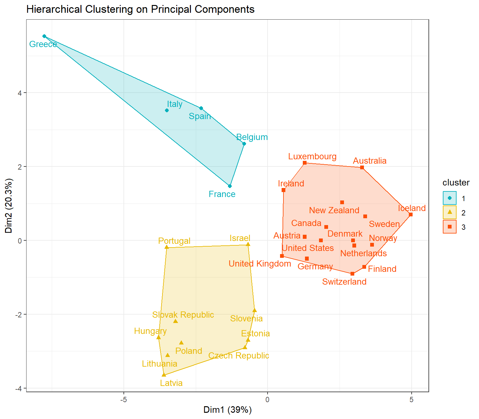
Let’s create a cluster plot based on HCPC using the factoextra package.
# Create cluster plot based on HCPC
fviz_cluster(
  dat.hcpc,
  repel = TRUE,
  show.clust.cent = FALSE,
  show.legend.text = FALSE,
  pointsize = 1.8,
  labelsize = 11,
  palette = c("#00AFBB", "#E7B800", "#FC4E07"),
  ggtheme = theme_minimal(),
  main = 'Hierarchical Clustering on Principal Components'
) +
theme_bw()
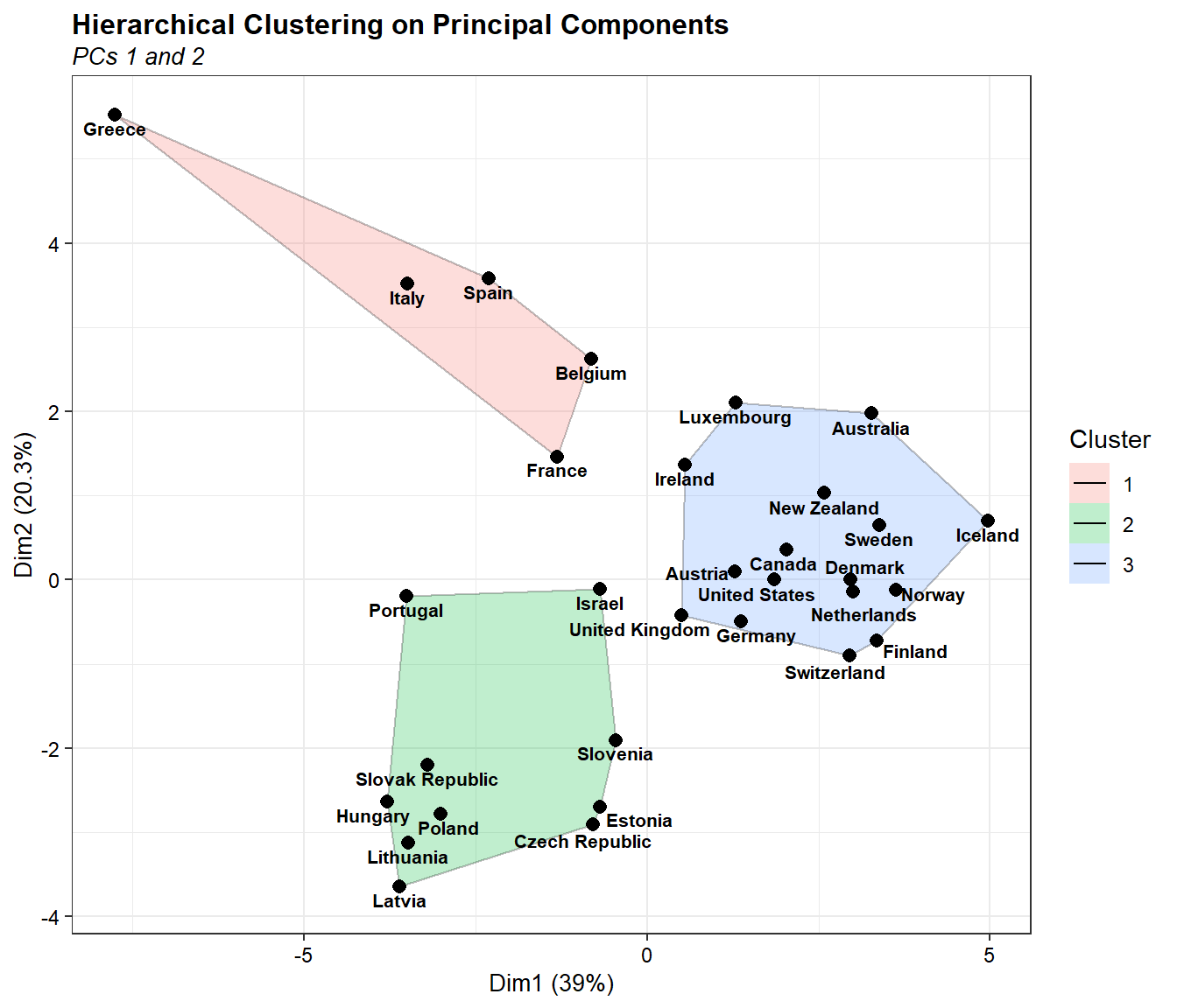
Now let’s create a cluster plot based on HCPC using the ggplot2 package and the ggalt package.
# Create cluster plot using ggplot2
library(ggplot2)
library(ggalt)
library(ggrepel)

ggplot(data = dat.norm, aes(x = Dim.1, y = Dim.2)) +
  geom_encircle(aes(fill = clust), alpha = 0.25, s_shape = 1, expand = 0) +
  geom_point(shape = 16, size = 2.5) +
  geom_text_repel(data = dat.norm,
                  aes(x = Dim.1, y = Dim.2, label = rownames(dat.norm)),
                  size = 2.8, segment.size = 0.1,
                  nudge_x = 0, nudge_y = -0.1,
                  color = 'black', fontface = 'bold',
                  seed = 123, max.overlaps = 30,
                  box.padding = unit(0.1, 'lines'),
                  point.padding = unit(0.1, 'lines')) +
  labs(title = 'Hierarchical Clustering on Principal Components',
       subtitle = 'PCs 1 and 2',
       fill = 'Cluster',
       x = paste0('Dim1 (', round(dat.pca$eig[1,2], 1), '%)'),
       y = paste0('Dim2 (', round(dat.pca$eig[2,2], 1), '%)')) +
  scale_color_brewer(palette = 'Set1') +
  theme_bw() +
  theme(plot.title = element_text(margin = margin(b = 3), size = 12,
                       hjust = 0, color = 'black', face = 'bold'),
        plot.subtitle = element_text(margin = margin(b = 3), size = 10,
                          hjust = 0, color = 'black', face = 'italic'),
        axis.title = element_text(size = 10, color = 'black'),
        axis.text = element_text(size = 9, color = 'black'))
References
Horn, J.L. 1965. A rationale and a test for the number of factors in factor analysis. Psychometrika, 30, 179-185.
Kaufman, L. and Rousseeuw, P.J. 1990. Finding Groups in Data: An Introduction to Cluster Analysis. Wiley, New York.
Tibshirani, R., Walther, G. and Hastie, T. 2001. Estimating the number of data clusters via the Gap statistic. Journal of the Royal Statistical Society B, 63, 411-423.
- Posted on:
- August 20, 2023
- Length:
- 29 minute read, 5979 words
- See Also: