Analyses of Pesticide Concentrations in California Surface Waters
By Charles Holbert
September 16, 2023
Introduction
Monitoring pesticide concentrations in surface waters is important for public authorities given the major concerns for environmental safety and the likelihood for increased public health risks. Since 1990, California has required detailed reporting for nearly all types of agricultural pesticide use and many nonagricultural pesticide uses as well. The Department of Pesticide Regulation’s (DPR) Surface Water Database (SURF) was developed under a 1997 agreement with the State Water Resource Control Board. The purpose of the database is to collect and make available information concerning the presence of pesticides in California surface waters.
Pesticide monitoring data often contain a substantial number of samples where concentrations are below levels of quantification (left-censored values or non-detects) for the analytical methods employed. In this post, established statistical techniques for handling left-censored data, including the Kaplan-Meier (KM) product-limit estimator (Kaplan and Meier 1958), robust regression on order statistics (rROS)(Helsel 2012), and maximum-likelihood estimation (MLE), will be used to analyze pesticide concentrations in heavily censored data sets. Analyses will be conducted using the R language for statistical computing and visualization.
Preliminaries
We’ll start by loading the main R libraries that will be used for data processing, visualization, and statistical analyses. There are several R packages that can be used for the statistical analyses of environmental data containing left-censored results. One package is EnvStats, which was developed by Steven P. Millard. A user manual (Millard 2013) is available that provides information on environmental statistics and documentation of the methods and procedures used in the EnvStats package. Two other packages are NADA, developed by Lopaka Lee and Dennis Helsel, and NADA2, developed by Paul Julian and Dennis Helsel. This two packages contain procedures documented in Statistics for Censored Environmental Data Using Minitab and R (Helsel 2012).
# Load libraries
library(dplyr)
library(lubridate)
library(tidyr)
library(ggplot2)
library(scales)
library(NADA)
library(NADA2)
library(EnvStats)
library(kableExtra)
Load Data
SURF contains data from a wide variety of environmental monitoring studies designed to test for the presence or absence of pesticides in California surface waters. The data represent concentrations of pesticide active ingredients or breakdown products measured in surface water samples collected between June 1925 and May 2022 from California rivers, creeks, agricultural drains, urban streams, and estuaries. SURF is freely accessible to the public.
Let’s load the surface water data that I previously downloaded from SURF.
# Load data
datin <- read.csv('data/surf_water_2023.csv', header = T)
Let’s inspect the general structure of the data.
# Inspect data
glimpse(datin)
## Rows: 1,046,243
## Columns: 17
## $ County                        <chr> "Sacramento", "Contra Costa", "Colusa", …
## $ Site_code                     <chr> "34_25", "07_117", "06_4", "40_36", "34_…
## $ Site_name                     <chr> "Arcade C Nr Del Paso Heights California…
## $ Latitude                      <dbl> 38.64196, 37.82571, 39.21431, 35.49293, …
## $ Longitude                     <dbl> -121.3820, -122.0035, -122.0001, -120.66…
## $ Sample_date                   <chr> "8/8/1997", "4/26/2017", "2/11/2001", "3…
## $ Chemical_name                 <chr> "ethyl parathion", "disulfoton sulfone",…
## $ Concentration..ppb.           <dbl> 0, 0, 0, 0, 0, 0, 0, 0, 0, 0, 0, 0, 0, 0…
## $ Level_of_quantification..ppb. <dbl> 0.0040, 0.0090, 0.0200, 0.1490, 0.0056, …
## $ Method_detection_level..ppb.  <dbl> -999.0000, -999.0000, -999.0000, -999.00…
## $ Sample_type                   <chr> "Filtered water sample", "Filtered water…
## $ Study_cd                      <int> 263, 263, 263, 263, 263, 263, 263, 263, …
## $ Study_description             <chr> "USGS NWIS water column data, downloaded…
## $ Study_weblink                 <chr> "https://waterdata.usgs.gov/nwis", "http…
## $ Data.source                   <chr> "USGS", "USGS", "USGS", "USGS", "USGS", …
## $ Agency                        <chr> "U.S. Geological Survey Water Resources …
## $ Record_id                     <int> 7897663, 8088243, 7883746, 8126506, 8111…
We see that there are 17 variables and over 1 million records. Let’s process the data so that it can quickly be parsed and analyzed. This includes renaming of variables to avoid potential naming convention errors during the analyses. Additionally, let’s add decimal date and calendar year variables.
# Prep data
dat <- datin %>%
  mutate(
    Sample_date = as.POSIXct(Sample_date, format = '%m/%d/%Y'),
    Detected = ifelse(Concentration..ppb. == 0, 'N', 'Y'),
    Censored = ifelse(Concentration..ppb. == 0, TRUE, FALSE),
    Units = 'ppb',
    Date = decimal_date(Sample_date),
    Year = as.numeric(format(Sample_date, '%Y'))
  ) %>%
  rename(
    SiteCode = Site_code,
    SiteName = Site_name,
    lat = Latitude,
    long = Longitude,
    SampleDate = Sample_date,
    Chemical = Chemical_name,
    Result = Concentration..ppb.,
    PQL = Level_of_quantification..ppb.,
    MDL = Method_detection_level..ppb.,
    SampleType = Sample_type,
    StudyCD = Study_cd,
    Description = Study_description,
    Weblink = Study_weblink,
    Source = Data.source,
    Record = Record_id,
  ) %>%
  mutate(Result = ifelse(Detected == 'N', PQL, Result))
Inspect Data
Let’s inspect the general structure of the processed data.
# Inspect general structure of data
glimpse(dat)
## Rows: 1,046,243
## Columns: 22
## $ County      <chr> "Sacramento", "Contra Costa", "Colusa", "San Luis Obispo",…
## $ SiteCode    <chr> "34_25", "07_117", "06_4", "40_36", "34_5", "34_26", "39_1…
## $ SiteName    <chr> "Arcade C Nr Del Paso Heights California_USGS NAWQA site",…
## $ lat         <dbl> 38.64196, 37.82571, 39.21431, 35.49293, 38.45602, 38.50029…
## $ long        <dbl> -121.3820, -122.0035, -122.0001, -120.6640, -121.5013, -12…
## $ SampleDate  <dttm> 1997-08-08, 2017-04-26, 2001-02-11, 2017-03-16, 2019-05-2…
## $ Chemical    <chr> "ethyl parathion", "disulfoton sulfone", "carbofuran", "me…
## $ Result      <dbl> 0.0040, 0.0090, 0.0200, 0.1490, 0.0056, 0.0060, 0.0100, 0.…
## $ PQL         <dbl> 0.0040, 0.0090, 0.0200, 0.1490, 0.0056, 0.0060, 0.0100, 0.…
## $ MDL         <dbl> -999.0000, -999.0000, -999.0000, -999.0000, -999.0000, -99…
## $ SampleType  <chr> "Filtered water sample", "Filtered water sample", "Filtere…
## $ StudyCD     <int> 263, 263, 263, 263, 263, 263, 263, 263, 263, 263, 263, 263…
## $ Description <chr> "USGS NWIS water column data, downloaded from the NWIS web…
## $ Weblink     <chr> "https://waterdata.usgs.gov/nwis", "https://waterdata.usgs…
## $ Source      <chr> "USGS", "USGS", "USGS", "USGS", "USGS", "USGS", "USGS", "U…
## $ Agency      <chr> "U.S. Geological Survey Water Resources Discipline", "U.S.…
## $ Record      <int> 7897663, 8088243, 7883746, 8126506, 8111094, 7851597, 7883…
## $ Detected    <chr> "N", "N", "N", "N", "N", "N", "N", "N", "N", "N", "N", "N"…
## $ Censored    <lgl> TRUE, TRUE, TRUE, TRUE, TRUE, TRUE, TRUE, TRUE, TRUE, TRUE…
## $ Units       <chr> "ppb", "ppb", "ppb", "ppb", "ppb", "ppb", "ppb", "ppb", "p…
## $ Date        <dbl> 1997.600, 2017.315, 2001.112, 2017.203, 2019.386, 2001.849…
## $ Year        <dbl> 1997, 2017, 2001, 2017, 2019, 2001, 2001, 2017, 2013, 2006…
SURF states that the data include results as far back as June 1925. Let’s see the number of results for samples collected prior to 1970.
# Inspect results prior to 1970
dat %>%
  filter(Year < 1970) %>%
  dplyr::select(County, SampleDate, Chemical) %>%
  kbl() %>%
  kable_minimal(full_width = F, position = "left")
| County | SampleDate | Chemical |
|---|---|---|
| Estuary | 1950-01-01 | chlorthal-dimethyl |
| Estuary | 1950-01-01 | alpha-endosulfan |
| Estuary | 1950-01-01 | diazinon |
| Estuary | 1950-01-01 | endosulfan sulfate |
| Estuary | 1950-01-01 | 2-hydroxycyclohexyl hexazinone |
| Estuary | 1950-01-01 | oxadiazon |
| Estuary | 1950-01-01 | lindane (gamma-bhc) |
| Estuary | 1950-01-01 | methoxychlor |
| Estuary | 1950-01-01 | chlorpyrifos |
| Estuary | 1950-01-01 | endosulfan ii |
| San Diego | 1950-01-01 | alpha-endosulfan |
| San Diego | 1950-01-01 | alpha-endosulfan |
| San Diego | 1950-01-01 | endosulfan ii |
| San Diego | 1950-01-01 | methoxychlor |
| San Diego | 1950-01-01 | endosulfan sulfate |
| San Diego | 1950-01-01 | methoxychlor |
| San Diego | 1950-01-01 | lindane (gamma-bhc) |
| San Diego | 1950-01-01 | endosulfan sulfate |
| San Diego | 1950-01-01 | endosulfan ii |
| San Diego | 1950-01-01 | alpha-endosulfan |
| San Diego | 1950-01-01 | lindane (gamma-bhc) |
| San Diego | 1950-01-01 | methoxychlor |
| San Diego | 1950-01-01 | methoxychlor |
| San Diego | 1950-01-01 | endosulfan sulfate |
| San Diego | 1950-01-01 | 2-hydroxycyclohexyl hexazinone |
| San Diego | 1950-01-01 | lindane (gamma-bhc) |
| San Diego | 1950-01-01 | 2-hydroxycyclohexyl hexazinone |
| San Diego | 1950-01-01 | lindane (gamma-bhc) |
| San Diego | 1950-01-01 | endosulfan ii |
| San Diego | 1950-01-01 | alpha-endosulfan |
| San Diego | 1950-01-01 | lindane (gamma-bhc) |
| San Diego | 1950-01-01 | alpha-endosulfan |
| San Diego | 1950-01-01 | 2-hydroxycyclohexyl hexazinone |
| San Diego | 1950-01-01 | endosulfan sulfate |
| San Diego | 1950-01-01 | endosulfan ii |
| San Diego | 1950-01-01 | endosulfan sulfate |
| San Diego | 1950-01-01 | endosulfan ii |
| San Diego | 1950-01-01 | 2-hydroxycyclohexyl hexazinone |
| San Diego | 1950-01-01 | 2-hydroxycyclohexyl hexazinone |
| San Diego | 1950-01-01 | methoxychlor |
| Estuary | 1950-01-01 | diazinon |
| Estuary | 1950-01-01 | diazinon |
| Estuary | 1950-01-01 | chlorpyrifos |
| Estuary | 1950-01-01 | chlorpyrifos |
| Merced | 1925-06-27 | diazinon |
| Merced | 1925-06-27 | ethyl parathion |
| Merced | 1925-06-27 | malathion |
| Merced | 1925-06-27 | methoxychlor |
| Merced | 1925-06-27 | methyl parathion |
| Merced | 1925-06-27 | lindane (gamma-bhc) |
| Merced | 1925-06-27 | alpha-endosulfan |
Let’s use the skimr package to get a more detailed summary of the data.
# Summary of data using skimr
skimr::skim(dat)
| Name | dat |
| Number of rows | 1046243 |
| Number of columns | 22 |
| _______________________ | |
| Column type frequency: | |
| character | 11 |
| logical | 1 |
| numeric | 9 |
| POSIXct | 1 |
| ________________________ | |
| Group variables | None |
Variable type: character
| skim_variable | n_missing | complete_rate | min | max | empty | n_unique | whitespace |
|---|---|---|---|---|---|---|---|
| County | 0 | 1.00 | 4 | 15 | 0 | 57 | 0 |
| SiteCode | 0 | 1.00 | 4 | 7 | 0 | 3798 | 0 |
| SiteName | 0 | 1.00 | 2 | 113 | 0 | 3708 | 0 |
| Chemical | 0 | 1.00 | 3 | 68 | 0 | 409 | 0 |
| SampleType | 0 | 1.00 | 0 | 95 | 5857 | 11 | 0 |
| Description | 0 | 1.00 | 42 | 291 | 0 | 761 | 0 |
| Weblink | 19631 | 0.98 | 21 | 114 | 0 | 65 | 0 |
| Source | 0 | 1.00 | 3 | 5 | 0 | 6 | 0 |
| Agency | 0 | 1.00 | 7 | 99 | 0 | 171 | 0 |
| Detected | 0 | 1.00 | 1 | 1 | 0 | 2 | 0 |
| Units | 0 | 1.00 | 3 | 3 | 0 | 1 | 0 |
Variable type: logical
| skim_variable | n_missing | complete_rate | mean | count |
|---|---|---|---|---|
| Censored | 0 | 1 | 0.94 | TRU: 980540, FAL: 65703 |
Variable type: numeric
| skim_variable | n_missing | complete_rate | mean | sd | p0 | p25 | p50 | p75 | p100 | hist |
|---|---|---|---|---|---|---|---|---|---|---|
| lat | 0 | 1.00 | 36.95 | 2.05 | 32.55 | 35.36 | 37.54 | 38.40 | 42.01 | ▅▁▇▆▁ |
| long | 0 | 1.00 | -120.57 | 1.81 | -124.29 | -121.65 | -121.27 | -119.51 | -114.14 | ▁▇▁▂▁ |
| Result | 0 | 1.00 | 0.31 | 7.98 | 0.00 | 0.00 | 0.01 | 0.06 | 5500.00 | ▇▁▁▁▁ |
| PQL | 0 | 1.00 | 0.25 | 4.89 | 0.00 | 0.00 | 0.01 | 0.05 | 1000.00 | ▇▁▁▁▁ |
| MDL | 76128 | 0.93 | -297.62 | 457.00 | -999.00 | -999.00 | 0.00 | 0.01 | 200.00 | ▃▁▁▁▇ |
| StudyCD | 0 | 1.00 | 431.50 | 299.80 | 6.00 | 263.00 | 263.00 | 563.00 | 1253.00 | ▂▇▂▁▂ |
| Record | 0 | 1.00 | 6823847.64 | 2430242.53 | 3513.00 | 7408095.50 | 7672700.00 | 7939655.50 | 8201845.00 | ▁▁▁▁▇ |
| Date | 0 | 1.00 | 2010.68 | 7.72 | 1925.48 | 2005.57 | 2012.20 | 2017.24 | 2022.36 | ▁▁▁▂▇ |
| Year | 0 | 1.00 | 2010.24 | 7.69 | 1925.00 | 2005.00 | 2012.00 | 2017.00 | 2022.00 | ▁▁▁▂▇ |
Variable type: POSIXct
| skim_variable | n_missing | complete_rate | min | max | median | n_unique |
|---|---|---|---|---|---|---|
| SampleDate | 0 | 1 | 1925-06-27 | 2022-05-11 | 2012-03-13 | 5431 |
Let’s use the plot_missing() function from the DataExplorer package to examine the data for missing values.
# Inspect missing data using DataExplorer
DataExplorer::plot_missing(dat)
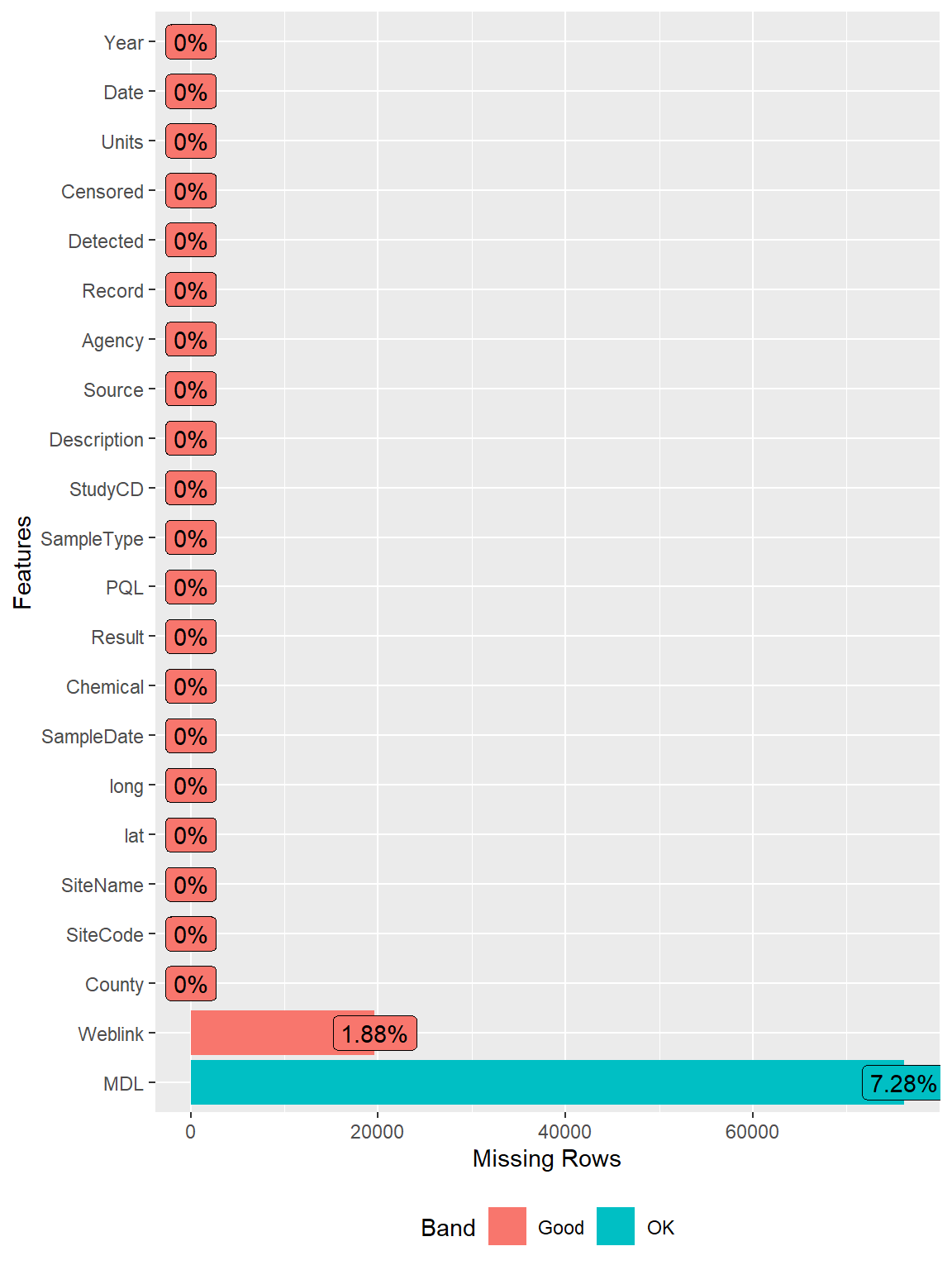
The variables “Weblink” and “MDL” contain missing values. Thus, let’s use the “PQL” variable for the non-detect censoring limit.
Duplicate Results
Duplicate sample results can provide valuable information about the level of measurement variability attributable to sampling and/or analytical techniques. However, duplicate results should not be used as separate observations in most statistical analyses, unless the test is specially structured to account for multiple data values per sampling event.
Let’s check the data for duplicate results based on site code, sample date, and chemical name.
# Check for duplicate results
dups <- dat[duplicated(dat[c('SiteCode', 'SampleDate', 'Chemical')]),]
glimpse(dups)
## Rows: 88,319
## Columns: 22
## $ County      <chr> "Santa Clara", "Riverside", "San Mateo", "Sonoma", "Marin"…
## $ SiteCode    <chr> "43_58", "33_2", "41_6", "49_89", "21_97", "43_41", "41_15…
## $ SiteName    <chr> "Saratoga C A Braemar Dr A Saratoga Ca", "Santa Ana R Bl P…
## $ lat         <dbl> 37.27220, 33.88335, 37.42361, 38.58741, 38.06950, 37.46023…
## $ long        <dbl> -122.0160, -117.6453, -122.1886, -122.8622, -122.5320, -12…
## $ SampleDate  <dttm> 2017-04-12, 2018-03-29, 2017-04-06, 2017-05-08, 2017-04-2…
## $ Chemical    <chr> "hexazinone degradates", "hexazinone degradates", "hexazin…
## $ Result      <dbl> 0.0760000, 0.0760000, 0.0220000, 0.2940000, 0.0020000, 0.0…
## $ PQL         <dbl> 7.60e-02, 7.60e-02, 2.20e-02, 2.94e-01, 2.00e-03, 1.00e-06…
## $ MDL         <dbl> -9.99e+02, -9.99e+02, -9.99e+02, -9.99e+02, -9.99e+02, 1.0…
## $ SampleType  <chr> "Filtered water sample", "Filtered water sample", "Filtere…
## $ StudyCD     <int> 263, 263, 263, 263, 263, 399, 408, 406, 408, 263, 407, 400…
## $ Description <chr> "USGS NWIS water column data, downloaded from the NWIS web…
## $ Weblink     <chr> "https://waterdata.usgs.gov/nwis", "https://waterdata.usgs…
## $ Source      <chr> "USGS", "USGS", "USGS", "USGS", "USGS", "CEDEN", "CEDEN", …
## $ Agency      <chr> "U.S. Geological Survey Water Resources Discipline", "U.S.…
## $ Record      <int> 8147068, 8143637, 8046765, 8151940, 8145641, 7442411, 7721…
## $ Detected    <chr> "N", "N", "N", "N", "N", "N", "Y", "Y", "Y", "N", "Y", "Y"…
## $ Censored    <lgl> TRUE, TRUE, TRUE, TRUE, TRUE, TRUE, FALSE, FALSE, FALSE, T…
## $ Units       <chr> "ppb", "ppb", "ppb", "ppb", "ppb", "ppb", "ppb", "ppb", "p…
## $ Date        <dbl> 2017.277, 2018.238, 2017.260, 2017.348, 2017.315, 1997.290…
## $ Year        <dbl> 2017, 2018, 2017, 2017, 2017, 1997, 2005, 2003, 2005, 2017…

# See proportion of results that are duplicates
length(dups$Result)/length(dat$Result)
## [1] 0.08441538
Let’s remove the duplicate results. For duplicate samples consisting of two detects, the sample with the maximum detected result will be selected. For duplicate samples consisting of two non-detects, the sample with the minimum quantification limit will be selected. For duplicates where there is one detect and one non-detect, the sample with the detected result will be selected.
# Assign zero to non-detects
dat <- dat %>%
  mutate(TC = ifelse(Detected == 'Y', Result, 0)) %>%
  droplevels()

# Sort the data
dat <- dat[with(dat, order(SiteCode, SampleDate, Chemical)), ]

# Create a variable that indicates a duplicate result
dat$DUP <- duplicated(dat[, c('SiteCode', 'SampleDate', 'Chemical')])

# This won't tell you that the first entry of the combination is a duplicate.
# Need to check the duplicate against the previous row
dat$DUP <- ifelse(
  duplicated(dat[, c('SiteCode', 'SampleDate', 'Chemical')], fromLast = T),
  yes = T, no = dat$DUP
)

# Remove duplicates
dat <- dat %>%
  group_by(SiteCode, SampleDate, Chemical, DUP) %>%
  mutate(Result = ifelse(sum(TC) == 0, min(PQL), max(TC))) %>%
  ungroup() %>%
  mutate(KEEP = ifelse(Result == PQL | Result == TC, 'Y', 'N')) %>%
  filter(KEEP == 'Y') %>%
  select(-TC, -DUP, -KEEP) %>%
  distinct(SiteCode, SampleDate, Chemical, Result, .keep_all = TRUE) %>%
  arrange(SiteCode, SampleDate, Chemical)
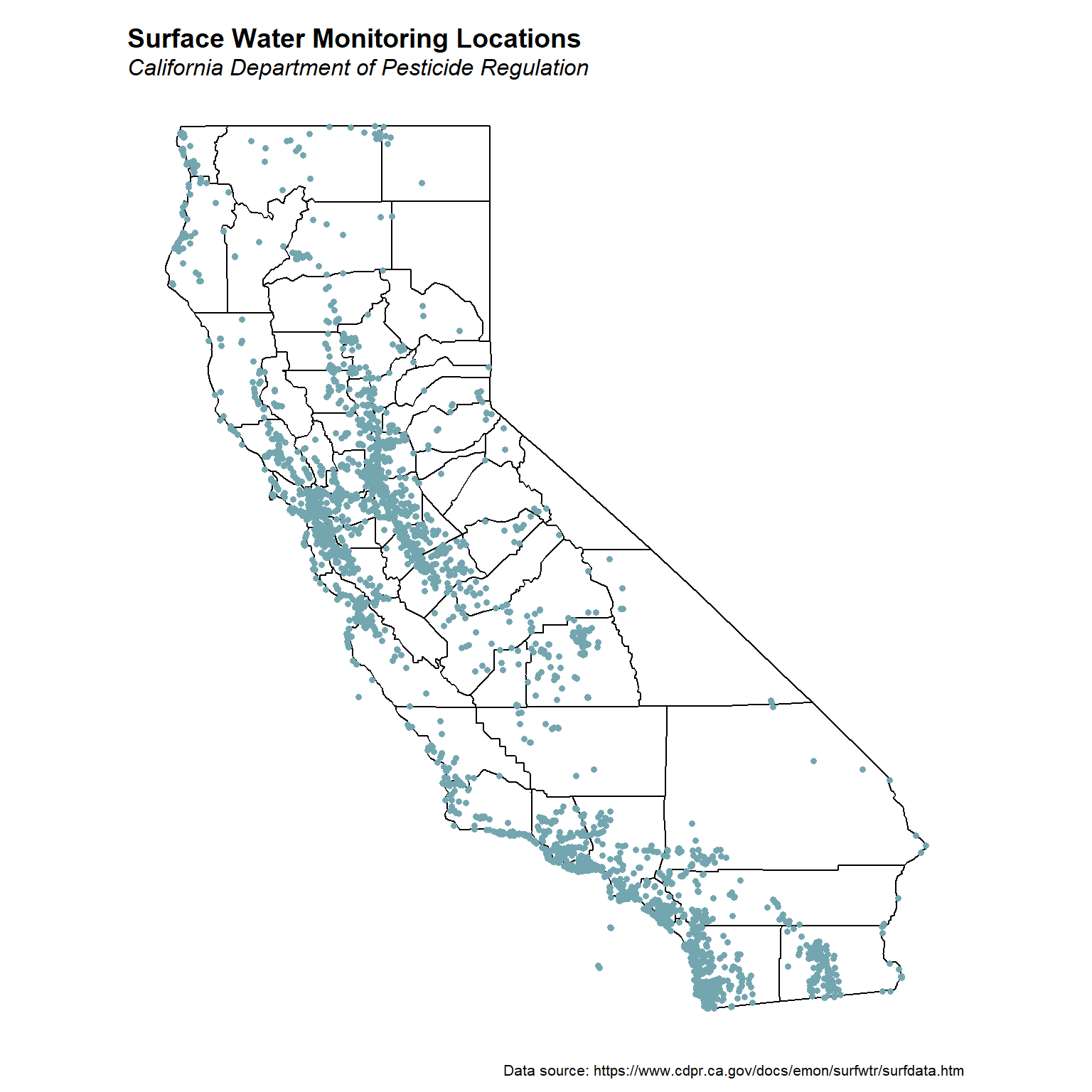
Sample Location Map
Let’s create a map showing the sample locations. We will use the maps and mapdata packages to get the state and counties boundary lines for California. The maps package contains outlines of many continents, countries, states, and counties. The mapdata package is a supplement to the maps package, providing some larger and/or higher-resolution databases. The maps package comes with a plotting function, but we will use the ggplot2 package to plot the map.
# Load libraries
library(mapdata)

# Get unique sampling locations
locs <- dat %>%
  dplyr::select(SiteCode) %>%
  distinct() %>%
  left_join(
    dat %>% dplyr::select(SiteCode, lat, long),
    by = 'SiteCode'
  )

# Get California state map
ca_df <- map_data('state') %>%
  filter(region == 'california')

# Gat California counties
ca_county <- map_data('county') %>%
  filter(region == 'california')

# Create map
ggplot() +
  geom_polygon(data = ca_county, aes(x = long, y = lat, group = group),
               fill = NA, color = 'black') +
  geom_polygon(data = ca_df, aes(x = long, y = lat, group = group),
               color = 'black', fill = NA) +
  geom_point(data = locs, aes(x = long, y = lat), color = '#74A6B0',
             shape = 16, size = 1.2) +
  coord_quickmap() +
  labs(title = 'Surface Water Monitoring Locations',
       subtitle = 'California Department of Pesticide Regulation',
       caption = 'Data source: https://www.cdpr.ca.gov/docs/emon/surfwtr/surfdata.htm',
       x = NULL,
       y = NULL) +
  theme_void() +
  theme(plot.title = element_text(margin = margin(b = 3), size = 14,
                       hjust = 0, color = 'black', face = 'bold'),
        plot.subtitle = element_text(margin = margin(b = 1), size = 12,
                              hjust = 0, color = 'black', face = 'italic'),
        plot.caption = element_text(size = 8, color = 'black'),
        plot.margin = unit(c(0.2, 0.1, 0.1, 0.1), 'in'))
Descriptive Statistics
Let’s calculate descriptive statistics for each of the pesticides. Descriptive statistics include the total number of samples, detected results, and frequency of detection; the minimum and maximum concentrations for detected and non-detected observations; and the mean, median, standard deviation, and coefficient of variation (CV) for each pesticide. The mean and median provide a measure of central tendency, while the standard deviation and CV provide a measure of variability in the data. The CV is the ratio of the sample standard deviation to the sample mean and thus indicates whether the amount of “spread” in the data is small or large relative to the average observed magnitude. Values less than one indicate that the standard deviation is smaller than the mean, while values greater than one occur when the standard deviation is greater than the mean. Descriptive statistics also include probabilities that the measured concentrations come from normal distributions as calculated by the Shapiro-Wilk test (1965). When the probability of the test is less than 0.05, the assumption of normality is rejected.
The mean and standard devaition are computed using both the KM and the rROS methods. If a data set is a mixture of detects and non-detects, but the non-detect fraction is no more than 50%, a censored estimation method such as the KM product-limit estimator or rROS can be used to compute adjusted estimates of the mean and standard deviation. When the censoring percentage is less than 50% and the sample size is small, either KM or rROS works reasonably well. For moderate to large censoring (e.g., 50% to 80%), rROS generally performs better than KM. Descriptive statistics are not calculated using the KM method for data sets with greater than 50% non-detects.
# Get descriptive statistics
cdat <- dat %>%
  group_by(Chemical) %>%
  summarize(
    UNITS   = unique(Units),
    OBS     = length(Result),
    DET     = length(Result[Detected == 'Y']),
    CEN     = length(Result[Detected == 'N']),
    PER.DET = round(DET*100/OBS, 2),
    MIN.CEN = tryCatch(min(Result[Detected == 'N'], na.rm = T),
                       warning = function(e) NA),
    MAX.CEN = tryCatch(max(Result[Detected == 'N'], na.rm = T),
                       warning = function(e) NA),
    MIN.DET = tryCatch(min(Result[Detected == 'Y'], na.rm = T),
                       warning = function(e) NA),
    MAX.DET = tryCatch(max(Result[Detected == 'Y'], na.rm = T),
                       warning = function(e) NA),
    LASTVAL  = Result[which.max(SampleDate)],
    LASTDATE = max(SampleDate),
    MEAN.KM = tryCatch(
      enparCensored(Result, Censored)$parameters['mean'],
      error = function(e) mean(Result, na.rm = T)
    ),
    MEDIAN.KM = tryCatch(
      median(
        ppointsCensored(Result, Censored, prob.method = 'kaplan-meier')$Order.Statistics
      ),
      error = function(e) median(Result, na.rm = T)
    ),
    SD.KM = tryCatch(
      enparCensored(Result, Censored)$parameters['sd'],
      error = function(e) sd(Result, na.rm = T)
    ),
    CV.KM = tryCatch(SD.KM/MEAN.KM, error = function(e) NA),
    MEAN.ROS = tryCatch(
      enormCensored(Result, Censored, method = 'rROS', lb.impute = 0)$parameters['mean'],
      error = function(e) mean(Result, na.rm = T)
    ),
    SD.ROS = tryCatch(
      enormCensored(Result, Censored, method = 'rROS', lb.impute = 0)$parameters['sd'],
      error = function(e) sd(Result, na.rm = T)
    ),
    SW.PVAL = tryCatch(shapiro.test(Result[Detected == 'Y'])$p.value,
                       error = function(e) NA)
  ) %>%
  ungroup()

# Change values if less than 4 observations or less than 50% detects
cdat$MEAN.KM[cdat$OBS < 4 | cdat$PER.DET < 50] <- NA
cdat$MEDIAN.KM[cdat$OBS < 4 | cdat$PER.DET < 50] <- NA
cdat$SD.KM[cdat$OBS < 4 | cdat$PER.DET < 50] <- NA
cdat$CV.KM[cdat$OBS < 4 | cdat$PER.DET < 50] <- NA
cdat$SW.PVAL[cdat$OBS < 4 | cdat$PER.DET < 50] <- NA

# Change values if less than 4 observations or less than 20% detects
cdat$MEAN.ROS[cdat$OBS < 4 | cdat$PER.DET < 20] <- NA
cdat$SD.ROS[cdat$OBS < 4 | cdat$PER.DET < 20] <- NA

# Print output
cdat
## # A tibble: 409 × 19
##    Chemical      UNITS   OBS   DET   CEN PER.DET MIN.CEN MAX.CEN MIN.DET MAX.DET
##    <chr>         <chr> <int> <int> <int>   <dbl>   <dbl>   <dbl>   <dbl>   <dbl>
##  1 1,3-dichloro… ppb     548     0   548    0     0.0038   3     NA       NA
##  2 1,4-dichloro… ppb     810     0   810    0     0.02    50     NA       NA
##  3 1-(3,4-dichl… ppb     435   122   313   28.0   0.003    1      0.0031   0.111
##  4 1h-1,2,4-tri… ppb     816    37   779    4.53  0.022    0.022  0.035    0.526
##  5 2,4,5-t       ppb      52     0    52    0     0.01     0.1   NA       NA
##  6 2,4-d         ppb    2776   793  1983   28.6   0.01   100      0.05    59
##  7 2,4-db        ppb     661     5   656    0.76  0.01    20      0.02     6.2
##  8 2,4-dichloro… ppb     243     0   243    0     0.36    50     NA       NA
##  9 2,4-xylenol   ppb      78     0    78    0     0.37    10     NA       NA
## 10 2,6-diethyla… ppb    2646     0  2646    0     0.0017   0.06  NA       NA
## # ℹ 399 more rows
## # ℹ 9 more variables: LASTVAL <dbl>, LASTDATE <dttm>, MEAN.KM <dbl>,
## #   MEDIAN.KM <dbl>, SD.KM <dbl>, CV.KM <dbl>, MEAN.ROS <dbl>, SD.ROS <dbl>,
## #   SW.PVAL <dbl>
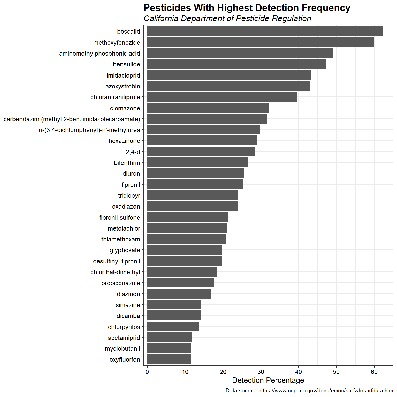
Most Detected Pesticides
Let’s create a list of the most detected pesticides for those pesticides with at least 1,000 samples, that have been detected at least 10% of the time, and that have been recently (since January 2020) analyzed.
# Get most detected pesticides
top_chem <- cdat %>%
  filter(
    OBS >= 1000 &
    PER.DET >= 10 &
    LASTDATE >= as.POSIXct('1/1/2020', format = '%m/%d/%Y')
  ) %>%
  droplevels() %>%
  arrange(-PER.DET, Chemical) %>%
  dplyr::select(Chemical, OBS, PER.DET, LASTDATE) %>%
  data.frame()

# Print list
top_chem %>%
  kbl() %>%
  kable_minimal(full_width = F, position = "left")
| Chemical | OBS | PER.DET | LASTDATE |
|---|---|---|---|
| boscalid | 1150 | 62.43 | 2022-03-29 |
| methoxyfenozide | 2110 | 60.00 | 2022-03-29 |
| aminomethylphosphonic acid | 1071 | 49.11 | 2021-09-02 |
| bensulide | 1000 | 47.20 | 2022-03-29 |
| imidacloprid | 3884 | 43.18 | 2022-04-28 |
| azoxystrobin | 3235 | 43.03 | 2022-03-29 |
| chlorantraniliprole | 1686 | 39.50 | 2022-03-29 |
| clomazone | 1071 | 32.03 | 2021-09-14 |
| carbendazim (methyl 2-benzimidazolecarbamate) | 1534 | 31.68 | 2021-10-19 |
| n-(3,4-dichlorophenyl)-n'-methylurea | 1504 | 29.72 | 2021-10-19 |
| hexazinone | 4451 | 29.14 | 2022-03-29 |
| 2,4-d | 2776 | 28.57 | 2022-03-16 |
| bifenthrin | 11155 | 26.64 | 2022-05-03 |
| diuron | 11329 | 25.55 | 2022-04-28 |
| fipronil | 4731 | 25.34 | 2022-05-03 |
| triclopyr | 2945 | 24.04 | 2022-03-16 |
| oxadiazon | 3599 | 23.84 | 2022-03-29 |
| fipronil sulfone | 4630 | 21.32 | 2022-05-03 |
| metolachlor | 3987 | 20.99 | 2021-10-19 |
| thiamethoxam | 2021 | 20.83 | 2022-04-28 |
| glyphosate | 5109 | 19.75 | 2022-04-28 |
| desulfinyl fipronil | 4412 | 19.72 | 2022-05-03 |
| chlorthal-dimethyl | 6667 | 18.36 | 2021-09-14 |
| propiconazole | 3352 | 17.63 | 2022-03-29 |
| diazinon | 25601 | 16.91 | 2022-05-03 |
| dicamba | 2711 | 14.13 | 2022-03-16 |
| simazine | 13981 | 14.13 | 2022-04-28 |
| chlorpyrifos | 27114 | 13.73 | 2022-05-03 |
| acetamiprid | 1775 | 11.77 | 2022-04-28 |
| myclobutanil | 2463 | 11.53 | 2021-10-19 |
| oxyfluorfen | 4902 | 11.46 | 2022-03-16 |
Let’s create a bar chart showing the most detected pesticides.
# Create bar chart
ggplot(data = top_chem, aes(x = PER.DET, y = reorder(Chemical, PER.DET))) +
  geom_col() +
  scale_x_continuous(limits = c(-1, 65),
                     breaks = seq(0, 65, by = 10),
                     expand = c(0, 0)) +
  labs(title = 'Pesticides With Highest Detection Frequency',
       subtitle = 'California Department of Pesticide Regulation',
       caption = 'Data source: https://www.cdpr.ca.gov/docs/emon/surfwtr/surfdata.htm',
       x = 'Detection Percentage',
       y = NULL) +
  theme_bw() +
  theme(plot.title = element_text(margin = margin(b = 3), size = 14,
                       hjust = 0, color = 'black', face = 'bold'),
        plot.subtitle = element_text(margin = margin(b = 3), size = 12,
                              hjust = 0, color = 'black', face = 'italic'),
        plot.caption = element_text(size = 8, color = 'black'),
        axis.title.y = element_text(size = 11, color = 'black'),
        axis.title.x = element_text(size = 11, color = 'black'),
        axis.text.x = element_text(size = 9, color = 'black'),
        axis.text.y = element_text(size = 9, color = 'black'))
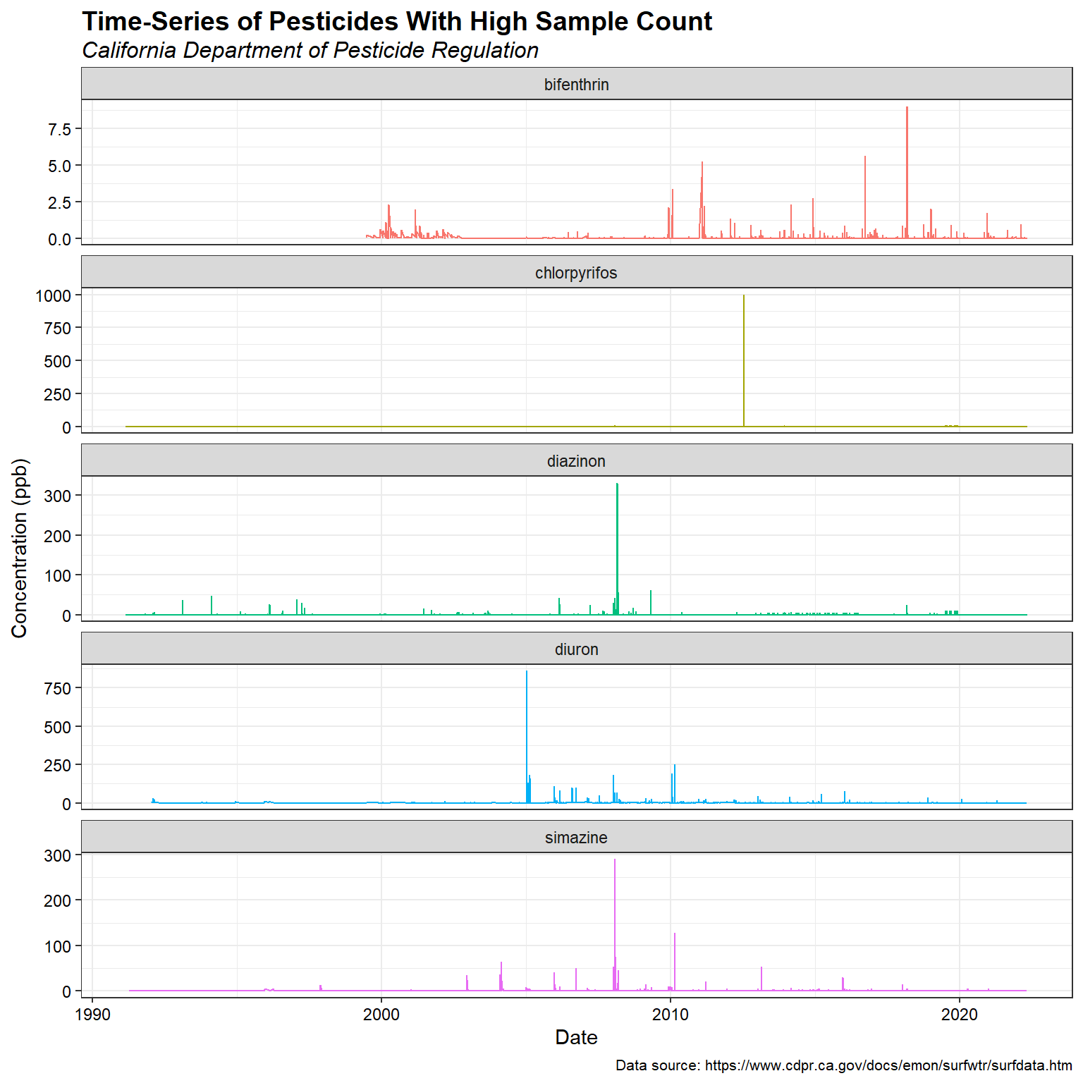
Let’s inspect the time series for a few pesticides that have a high sample count.
dat %>%
  filter(
    Year > 1990 &
    Chemical %in% c('bifenthrin', 'chlorpyrifos', 'diazinon', 'diuron', 'simazine')
  ) %>%
  ggplot(aes(x = Date, y = Result, color = Chemical)) +
    geom_line() +
    facet_wrap(~ Chemical, ncol = 1, scale = 'free_y') +
    labs(title = 'Time-Series of Pesticides With High Sample Count',
         subtitle = 'California Department of Pesticide Regulation',
         caption = 'Data source: https://www.cdpr.ca.gov/docs/emon/surfwtr/surfdata.htm',
         x = 'Date',
         y = 'Concentration (ppb)') +
    theme_bw() +
    theme(plot.title = element_text(margin = margin(b = 3), size = 14,
                         hjust = 0, color = 'black', face = 'bold'),
          plot.subtitle = element_text(margin = margin(b = 3), size = 12,
                            hjust = 0, color = 'black', face = 'italic'),
          plot.caption = element_text(size = 8, color = 'black'),
          axis.title.y = element_text(size = 11, color = 'black'),
          axis.title.x = element_text(size = 11, color = 'black'),
          axis.text.x = element_text(size = 9, color = 'black'),
          axis.text.y = element_text(size = 9, color = 'black'),
          legend.position = 'none')
Bifenthrin Data
Bifenthrin has been analyzed in a significant number of samples and has a low, but reasonable detection frequency when compared to the other pesticides. Let’s extract the bifenthrin data from the complete data set and use those data for further statistical analyses.
# Get bifenthrin data
bif <- dat %>%
  filter(Chemical == 'bifenthrin') %>%
  droplevels()
Let’s rename the categories of the “SampleType” variable to shorten them for ease of use in statistical analyses.
# Inspect sample type
sort(unique(bif$SampleType))
## [1] "Filtered water sample"
## [2] "Sample-type unknown"
## [3] "Single whole water sample"
## [4] "Whole water sample split through ten-port splitter into discrete samples"

# Function to change sample type names
change_names <- function(x) case_when(
  x == 'Filtered water sample' ~ 'Filtered',
  x == 'Sample-type unknown' ~ 'Unknown',
  x == 'Single whole water sample' ~ 'Single',
  x == 'Whole water sample split through ten-port splitter into discrete samples' ~ 'Split',
  TRUE ~ x
)

# Change sample type names
bif <- bif %>% mutate(SampleType = change_names(SampleType))
Sample Counts
Let’s calculate sample counts for the bifenthrin data by “SampleType.”
# Get counts by sample type
bif %>%
  group_by(SampleType) %>%
  summarize(
    OBS     = length(Result),
    DET     = length(Result[Detected == 'Y']),
    CEN     = length(Result[Detected == 'N']),
    PER.DET = round(DET*100/OBS, 2)
  ) %>%
  ungroup() %>%
  kbl() %>%
  kable_minimal(full_width = F, position = "left")
| SampleType | OBS | DET | CEN | PER.DET |
|---|---|---|---|---|
| Filtered | 1927 | 46 | 1881 | 2.39 |
| Single | 2658 | 1321 | 1337 | 49.70 |
| Split | 183 | 40 | 143 | 21.86 |
| Unknown | 6387 | 1565 | 4822 | 24.50 |
Let’s calculate sample counts for the bifenthrin data by “SampleType” and “Year.”
# Create two-way table of counts by sample type and year
xtabs(~ Year + SampleType, data = bif)
##       SampleType
## Year   Filtered Single Split Unknown
##   1999        0      0    25       0
##   2000        1      0    84       0
##   2001       11      0    47       0
##   2002        4      0    27       0
##   2003       44    132     0       0
##   2004        5     25     0     136
##   2005        6     28     0     318
##   2006       39      0     0     451
##   2007       12      3     0     577
##   2008       78     70     0     382
##   2009       75    170     0     231
##   2010       74    137     0     273
##   2011       33     83     0     320
##   2012       73    101     0     316
##   2013       78    118     0     458
##   2014       56    153     0     471
##   2015      131    239     0     211
##   2016      218    219     0     298
##   2017      580    157     0     233
##   2018      118    173     0     569
##   2019      191    215     0     417
##   2020       40    294     0     365
##   2021       60    301     0     344
##   2022        0     40     0      17
There are relatively few “Split” sample types in the bifenthrin data. Additionally, the “Split” samples were all collected between 1999 and 2002.
Post Plot
Let’s create a post plot of the maximum bifenthrin concentration for each sample location across the state, where the symbol sizes and colors are coded by concentration.
# Get max bifenthrin concentration by site
bif_max <- bif %>%
  group_by(SiteCode) %>%
  summarize(
    conc = max(Result)
  ) %>%
  left_join(
    bif %>% dplyr::select(SiteCode, lat, long),
    by = 'SiteCode'
  )

# Create color-scale for mapping bifenthrin concentrations
cols <- c(
  "#0000ff", "#0028d7", "#0050af", "#007986", "#00a15e",
  "#00ca35", "#00f20d", "#1aff00", "#43ff00", "#6bff00",
  "#94ff00", "#bcff00", "#e5ff00", "#fff200", "#ffca00",
  "#ffa100", "#ff7900", "#ff5000", "#ff2800", "#ff0000"
)

# Create map of max bifenthrin concentrations
ggplot() +
  geom_polygon(data = ca_county, aes(x = long, y = lat, group = group),
               fill = NA, color = 'black') +
  geom_polygon(data = ca_df, aes(x = long, y = lat, group = group),
               color = 'black', fill = NA) +
  geom_point(data = bif_max, aes(x = long, y = lat), color = '#74A6B0',
             shape = 16, size = 1.2) +
  geom_point(data = bif_max, aes(x = long, y = lat, color = log(conc), size = conc),
             shape = 16) +
  coord_quickmap() +
  scale_color_gradientn(colors = alpha(cols, alpha = 1)) +
#  scale_color_gradientn(colors = alpha(rev(brewer.pal(11, 'Spectral')), alpha = 1)) +
  guides(size = FALSE) +
  labs(title = 'Maximum Bifenthrin Surface Water Concentration',
       subtitle = 'California Department of Pesticide Regulation',
       caption = 'Data source: https://www.cdpr.ca.gov/docs/emon/surfwtr/surfdata.htm',
       color = 'Natural Log of \nConcentration\ngiven in ppb',
       x = NULL,
       y = NULL) +
  theme_void() +
  theme(plot.title = element_text(margin = margin(b = 3), size = 14,
                       hjust = 0, color = 'black', face = 'bold'),
        plot.subtitle = element_text(margin = margin(b = 1), size = 12,
                              hjust = 0, color = 'black', face = 'italic'),
        plot.caption = element_text(size = 8, color = 'black'),
        legend.position = c(0.9, 0.7),
        legend.title.align = 0,
        legend.title = element_text(size = 11),
        legend.text = element_text(size = 10),
        plot.margin = unit(c(0.2, 0.1, 0.1, 0.1), 'in'))
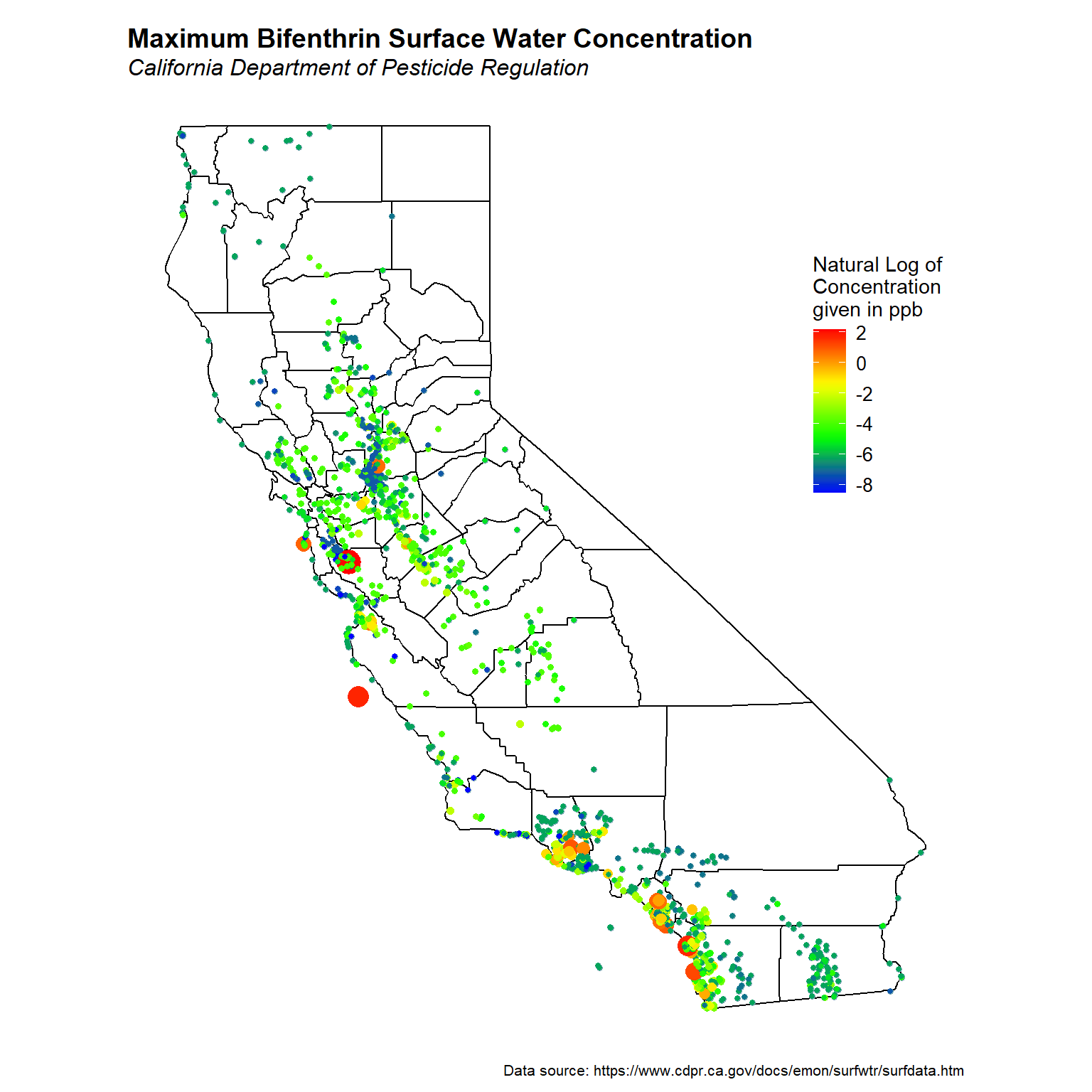
It appears that the highest concentrations of bifenthrin occur along the coast, mainly in central and southern California.
Detections by County
Let’s create a plot of bifenthrin detection frequency by county, where the symbol sizes and colors are coded by concentration.
# Plot of bifenthrin detection frequency by county
bif %>%
  dplyr::select(County, Detected) %>%
  count(County, Detected) %>%
  tidyr::drop_na() %>%
  group_by(County) %>%
  mutate(percent_detect = 100*n/sum(n)) %>%
  ungroup() %>%
  filter(Detected == 'Y') %>%
  ggplot(aes(x = percent_detect, y = County, col = percent_detect, size = n)) +
    geom_point() +
    scale_x_continuous(limits = c(-1, 101),
                       breaks = seq(0, 100, by = 20),
                       expand = c(0, 0)) +
    scale_y_discrete(limits = rev) +
    scale_color_gradientn(colors = alpha(cols, alpha = 1)) +
    labs(title = 'Bifenthrin Surface Water Detections by County',
         subtitle = 'California Department of Pesticide Regulation',
         caption = 'Data source: https://www.cdpr.ca.gov/docs/emon/surfwtr/surfdata.htm',
         color = 'Detected',
         size = 'Samples',
         x = 'Detection Percentage',
         y = 'County') +
    theme_bw() +
    theme(plot.title = element_text(margin = margin(b = 3), size = 12,
                         hjust = 0, color = 'black', face = 'bold'),
          plot.subtitle = element_text(margin = margin(b = 3), size = 11,
                            hjust = 0, color = 'black', face = 'italic'),
          plot.caption = element_text(size = 8, color = 'black'),
          axis.title = element_text(size = 11, color = 'black'),
          axis.text = element_text(size = 9, color = 'black'))
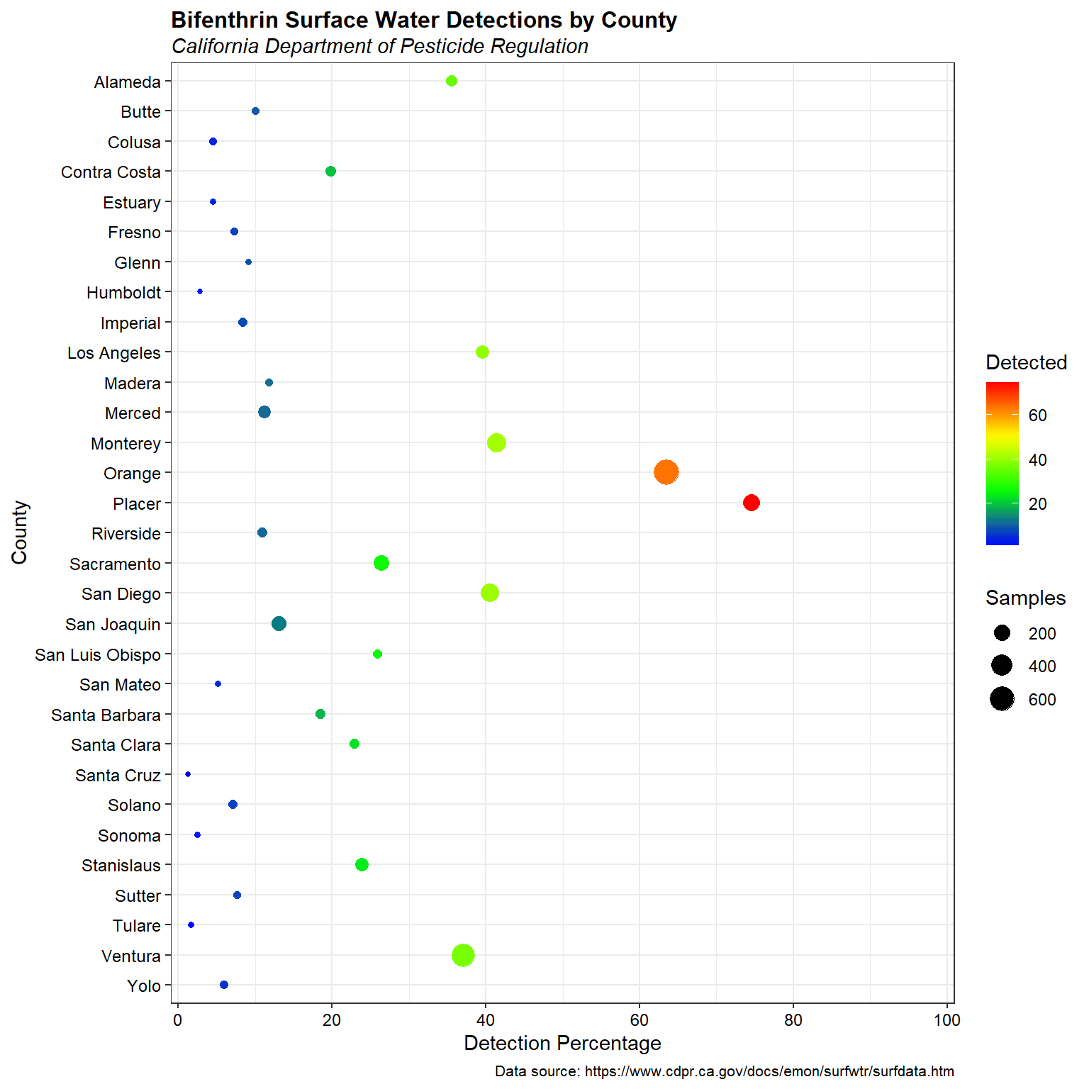
The highest concentrations of bifenthrin occur in Orange and Placer counties.
Outliers
Extreme outliers can adversely affect the results of statistical calculations. An outlier plot of bifenthrin concentrations is provided below. Outlier plots show the concentrations of a constituent in relationship to a measure of central tendency of the data and two nonparametric limits designed to assist in outlier identification. These limits are estabished using the box plot method and the Hampel identifier (Wilcox 2010). Observations too far from the median of the data with respect to their interquartile range (IQR) and Median Absolute Deviation (MAD) are declared to be statistical outliers.
# Load functions
source('functions/helper_functions.R')
source('functions/outlier_plot.R')

# Create outlier plot
with(bif,
  outlier_plot(
    x = Result,
    xcen = Detected,
    param = 'bifenthrin',
    Log = TRUE
  )
)
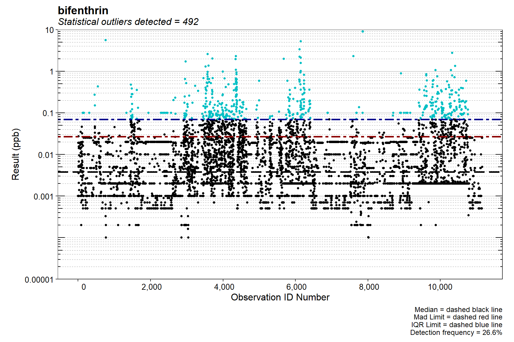
Although many samples are identified as statistical outliers, it’s likely that very few are actual, physical outliers.
Data Distribution
We can choose the best fitting distribution to our data using the distChooseCensored() function in the EnvStats package. The distChooseCensored() function performs a series of goodness-of-fit tests for censored data from a set of candidate probability distributions to determine which probability distribution provides the best fit for a data set.
# Goodness-of-fit tests using EnvStats
bif_gof <- with(bif,
  distChooseCensored(
    x = Result, censored = Censored,
    alpha = 0.05, method = 'sf',
    choices = c('norm', 'gamma', 'lnorm'),
    prob.method = 'hirsch-stedinger',
    keep.data = FALSE
  )
)
print(bif_gof)
## $choices
## [1] "Normal"    "Gamma"     "Lognormal"
##
## $method
## [1] "Shapiro-Francia"
##
## $decision
## [1] "Nonparametric"
##
## $alpha
## [1] 0.05
##
## $distribution.parameters
## NULL
##
## $estimation.method
## NULL
##
## $sample.size
## [1] 11155
##
## $censoring.side
## [1] "left"
##
## $censoring.levels
##  [1] 0.0001000 0.0001020 0.0001610 0.0002000 0.0003300 0.0005000 0.0007000
##  [8] 0.0007891 0.0010000 0.0010400 0.0010964 0.0011800 0.0012000 0.0012205
## [15] 0.0012316 0.0014300 0.0014500 0.0015000 0.0015800 0.0016400 0.0017800
## [22] 0.0020000 0.0020400 0.0020600 0.0020619 0.0020833 0.0020900 0.0020942
## [29] 0.0021000 0.0021053 0.0021100 0.0021277 0.0021300 0.0021500 0.0021700
## [36] 0.0022000 0.0022200 0.0022300 0.0022500 0.0023000 0.0023300 0.0024400
## [43] 0.0024691 0.0025000 0.0025400 0.0030000 0.0031700 0.0040000 0.0047000
## [50] 0.0050000 0.0053000 0.0064400 0.0065500 0.0068500 0.0074900 0.0079300
## [57] 0.0100000 0.0147000 0.0153000 0.0169000 0.0190000 0.0200000 0.0250000
## [64] 0.0400000 0.0500000 0.1000000 2.0000000 2.3121387 9.0000000
##
## $percent.censored
## [1] 73.35724
##
## $test.results
## $test.results$norm
##
## Results of Goodness-of-Fit Test
## Based on Type I Censored Data
## -------------------------------
##
## Test Method:                     Shapiro-Francia GOF
##                                  (Multiply Censored Data)
##
## Hypothesized Distribution:       Normal
##
## Censoring Side:                  left
##
## Censoring Level(s):              0.0001000 0.0001020 0.0001610 0.0002000 0.0003300 0.0005000 0.0007000 0.0007891 0.0010000 0.0010400 0.0010964 0.0011800 0.0012000 0.0012205 0.0012316 0.0014300 0.0014500 0.0015000 0.0015800 0.0016400 0.0017800 0.0020000 0.0020400 0.0020600 0.0020619 0.0020833 0.0020900 0.0020942 0.0021000 0.0021053 0.0021100 0.0021277 0.0021300 0.0021500 0.0021700 0.0022000 0.0022200 0.0022300 0.0022500 0.0023000 0.0023300 0.0024400 0.0024691 0.0025000 0.0025400 0.0030000 0.0031700 0.0040000 0.0047000 0.0050000 0.0053000 0.0064400 0.0065500 0.0068500 0.0074900 0.0079300 0.0100000 0.0147000 0.0153000 0.0169000 0.0190000 0.0200000 0.0250000 0.0400000 0.0500000 0.1000000 2.0000000 2.3121387 9.0000000
##
## Estimated Parameter(s):          mean = -0.1947556
##                                  sd   =  0.2520999
##
## Estimation Method:               MLE
##
## Data:                            Result
##
## Censoring Variable:              Censored
##
## Sample Size:                     11155
##
## Percent Censored:                73.35724%
##
## Test Statistic:                  W = 0.3102312
##
## Test Statistic Parameters:       N     = 1.115500e+04
##                                  DELTA = 7.335724e-01
##
## P-value:                         0
##
## Alternative Hypothesis:          True cdf does not equal the
##                                  Normal Distribution.
##
## $test.results$gamma
##
## Results of Goodness-of-Fit Test
## Based on Type I Censored Data
## -------------------------------
##
## Test Method:                     Shapiro-Francia GOF
##                                  (Multiply Censored Data)
##                                  Based on Chen & Balakrisnan (1995)
##
## Hypothesized Distribution:       Gamma
##
## Censoring Side:                  left
##
## Censoring Level(s):              0.0001000 0.0001020 0.0001610 0.0002000 0.0003300 0.0005000 0.0007000 0.0007891 0.0010000 0.0010400 0.0010964 0.0011800 0.0012000 0.0012205 0.0012316 0.0014300 0.0014500 0.0015000 0.0015800 0.0016400 0.0017800 0.0020000 0.0020400 0.0020600 0.0020619 0.0020833 0.0020900 0.0020942 0.0021000 0.0021053 0.0021100 0.0021277 0.0021300 0.0021500 0.0021700 0.0022000 0.0022200 0.0022300 0.0022500 0.0023000 0.0023300 0.0024400 0.0024691 0.0025000 0.0025400 0.0030000 0.0031700 0.0040000 0.0047000 0.0050000 0.0053000 0.0064400 0.0065500 0.0068500 0.0074900 0.0079300 0.0100000 0.0147000 0.0153000 0.0169000 0.0190000 0.0200000 0.0250000 0.0400000 0.0500000 0.1000000 2.0000000 2.3121387 9.0000000
##
## Estimated Parameter(s):          shape = 0.0809592
##                                  scale = 0.1996473
##
## Estimation Method:               MLE
##
## Data:                            Result
##
## Censoring Variable:              Censored
##
## Sample Size:                     11153
##
## Percent Censored:                73.35246%
##
## Test Statistic:                  W = 0.8867182
##
## Test Statistic Parameters:       N     = 1.115300e+04
##                                  DELTA = 7.335246e-01
##
## P-value:                         0
##
## Alternative Hypothesis:          True cdf does not equal the
##                                  Gamma Distribution.
##
## $test.results$lnorm
##
## Results of Goodness-of-Fit Test
## Based on Type I Censored Data
## -------------------------------
##
## Test Method:                     Shapiro-Francia GOF
##                                  (Multiply Censored Data)
##
## Hypothesized Distribution:       Lognormal
##
## Censoring Side:                  left
##
## Censoring Level(s):              0.0001000 0.0001020 0.0001610 0.0002000 0.0003300 0.0005000 0.0007000 0.0007891 0.0010000 0.0010400 0.0010964 0.0011800 0.0012000 0.0012205 0.0012316 0.0014300 0.0014500 0.0015000 0.0015800 0.0016400 0.0017800 0.0020000 0.0020400 0.0020600 0.0020619 0.0020833 0.0020900 0.0020942 0.0021000 0.0021053 0.0021100 0.0021277 0.0021300 0.0021500 0.0021700 0.0022000 0.0022200 0.0022300 0.0022500 0.0023000 0.0023300 0.0024400 0.0024691 0.0025000 0.0025400 0.0030000 0.0031700 0.0040000 0.0047000 0.0050000 0.0053000 0.0064400 0.0065500 0.0068500 0.0074900 0.0079300 0.0100000 0.0147000 0.0153000 0.0169000 0.0190000 0.0200000 0.0250000 0.0400000 0.0500000 0.1000000 2.0000000 2.3121387 9.0000000
##
## Estimated Parameter(s):          meanlog = -7.955304
##                                  sdlog   =  3.085124
##
## Estimation Method:               MLE
##
## Data:                            Result
##
## Censoring Variable:              Censored
##
## Sample Size:                     11155
##
## Percent Censored:                73.35724%
##
## Test Statistic:                  W = 0.9861763
##
## Test Statistic Parameters:       N     = 1.115500e+04
##                                  DELTA = 7.335724e-01
##
## P-value:                         3.183791e-09
##
## Alternative Hypothesis:          True cdf does not equal the
##                                  Lognormal Distribution.
##
##
## $data.name
## [1] "Result"
##
## $censoring.name
## [1] "Censored"
##
## attr(,"class")
## [1] "distChooseCensored"
The distChooseCensored() function indicates that the bifenthrin data do not follow a normal, lognornal, or gamma distribution. The recommended decision is to assume no distribution and use nonparametric statistical methods.
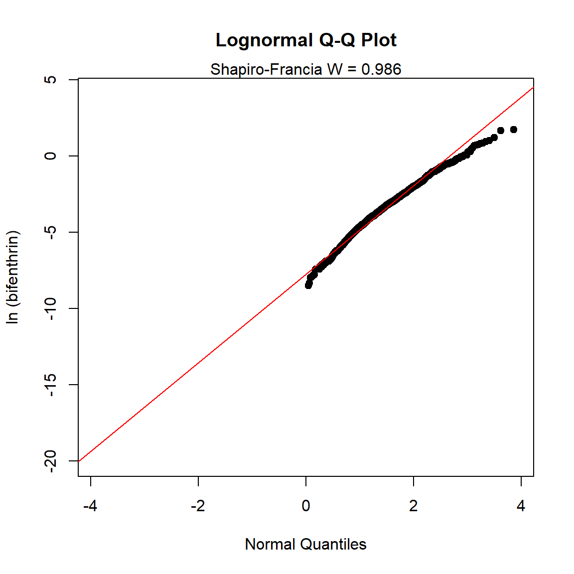
Another option is to use the cenCompareQQ() function in the NADA2 package. The cenCompareQQ() function plots three censored quantile-quantile (Q-Q) plots based on normal, lognormal, and gamma distributions and prints the best-fit distribution. The distribution with the highest Shapiro-Francia test statistic (W) is selected as the best fit of the three distrbutions.
# Goodness-of-fit tests using NADA2
with(bif, cenCompareQQ(
    x.var = Result,
    cens.var = Censored,
    Yname = 'bifenthrin'
  )
)
## Best of the three distributions is the lognormal
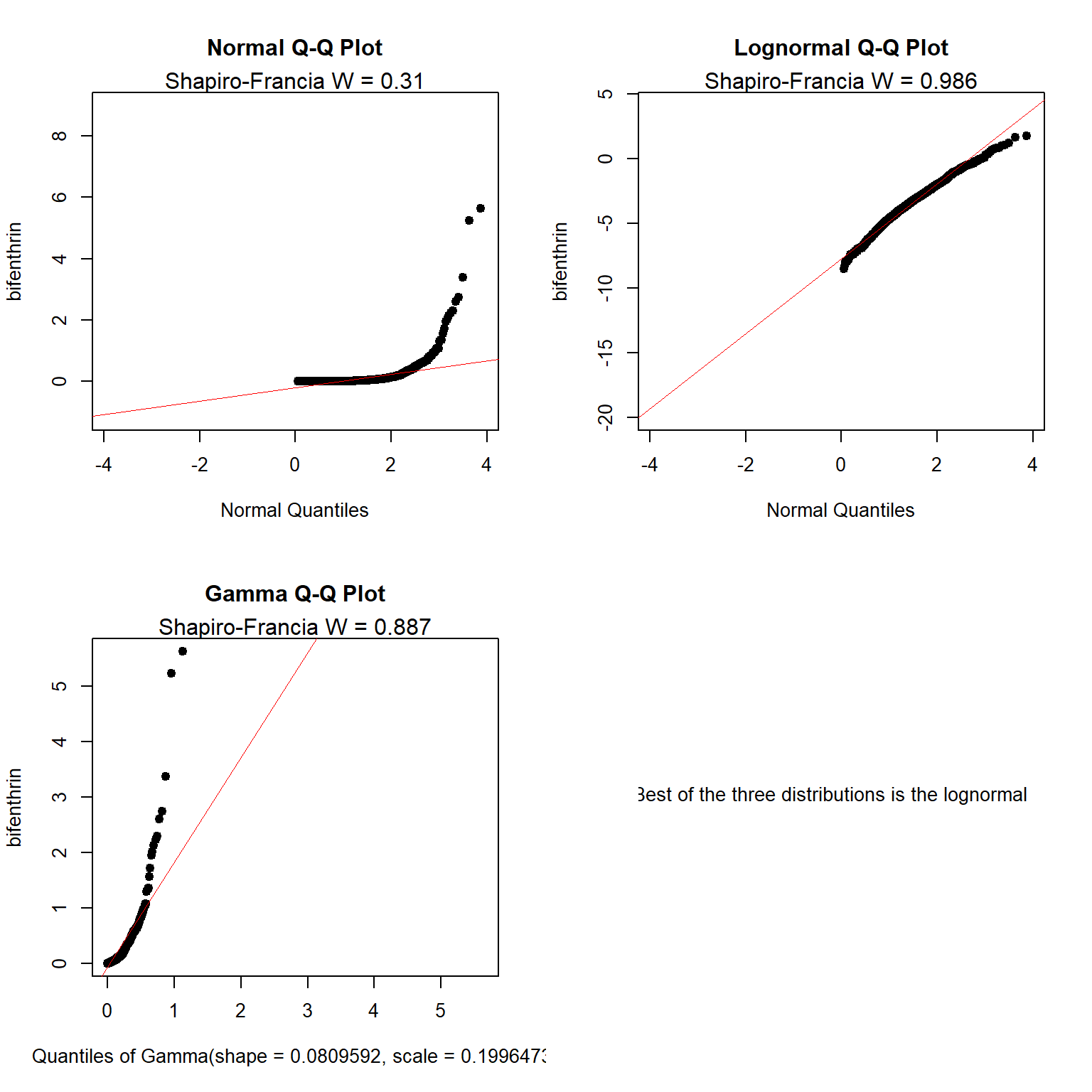
The cenCompareQQ() function indicates that the lognormal distribution is the best of the three distributions tested.
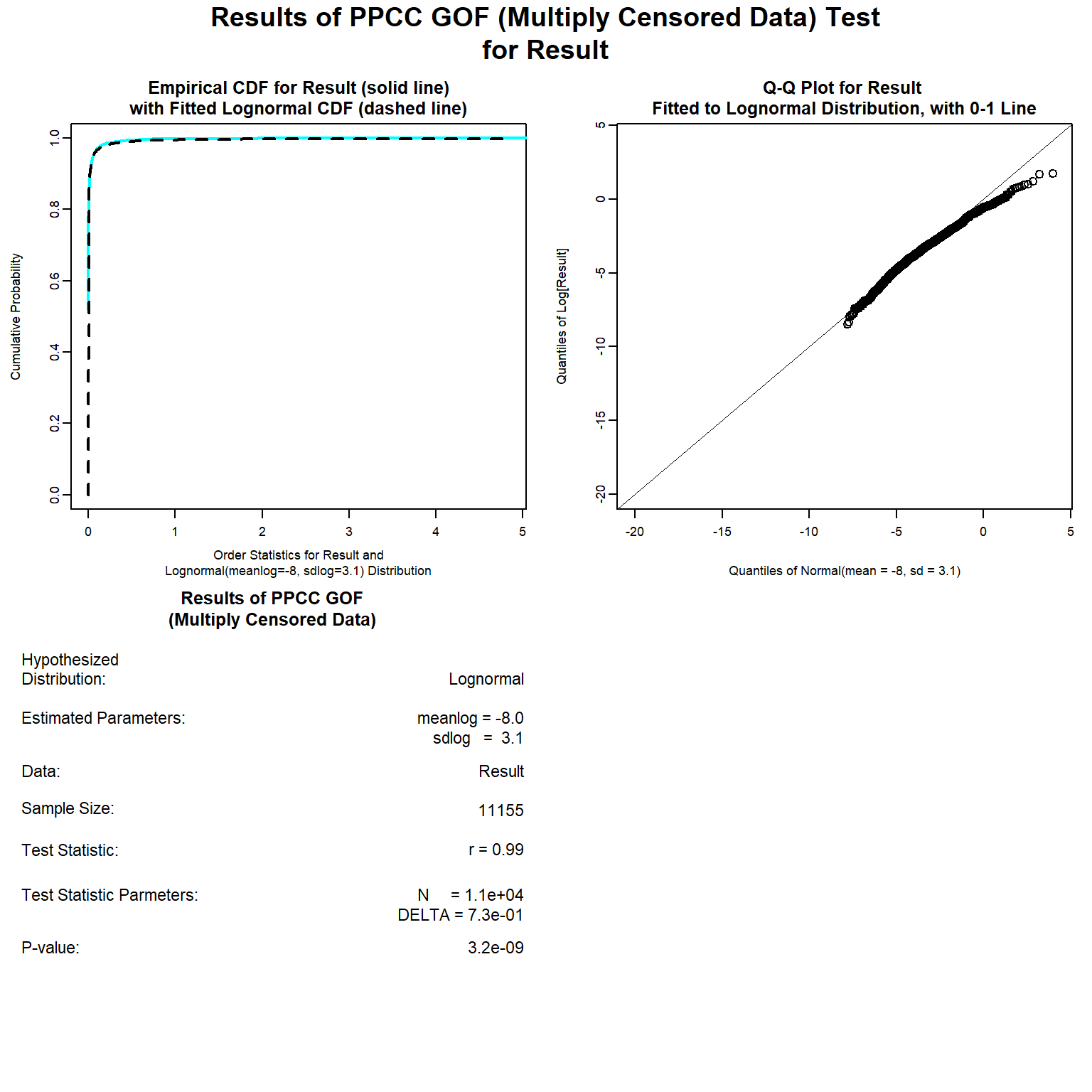
Let’s use the gofTestCensored() function in the EnvStats package to see how well a lognormal distribution fits the bifenthrin data.
# Goodness-of-fit test for lognormal distribution using EnvStats
bif_lnorm <- with(bif,
  gofTestCensored(
    x = Result, censored = Censored,
    test = 'ppcc', dist = 'lnorm'
  )
)
plot(bif_lnorm)
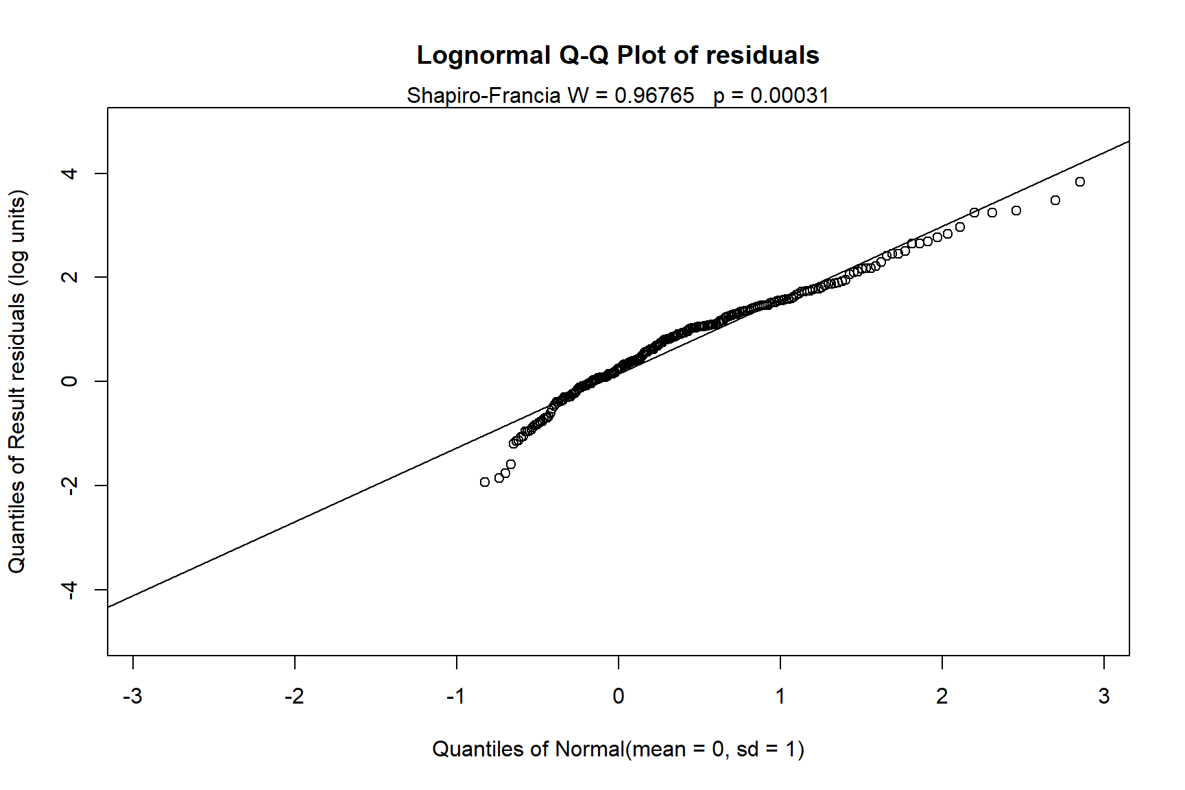
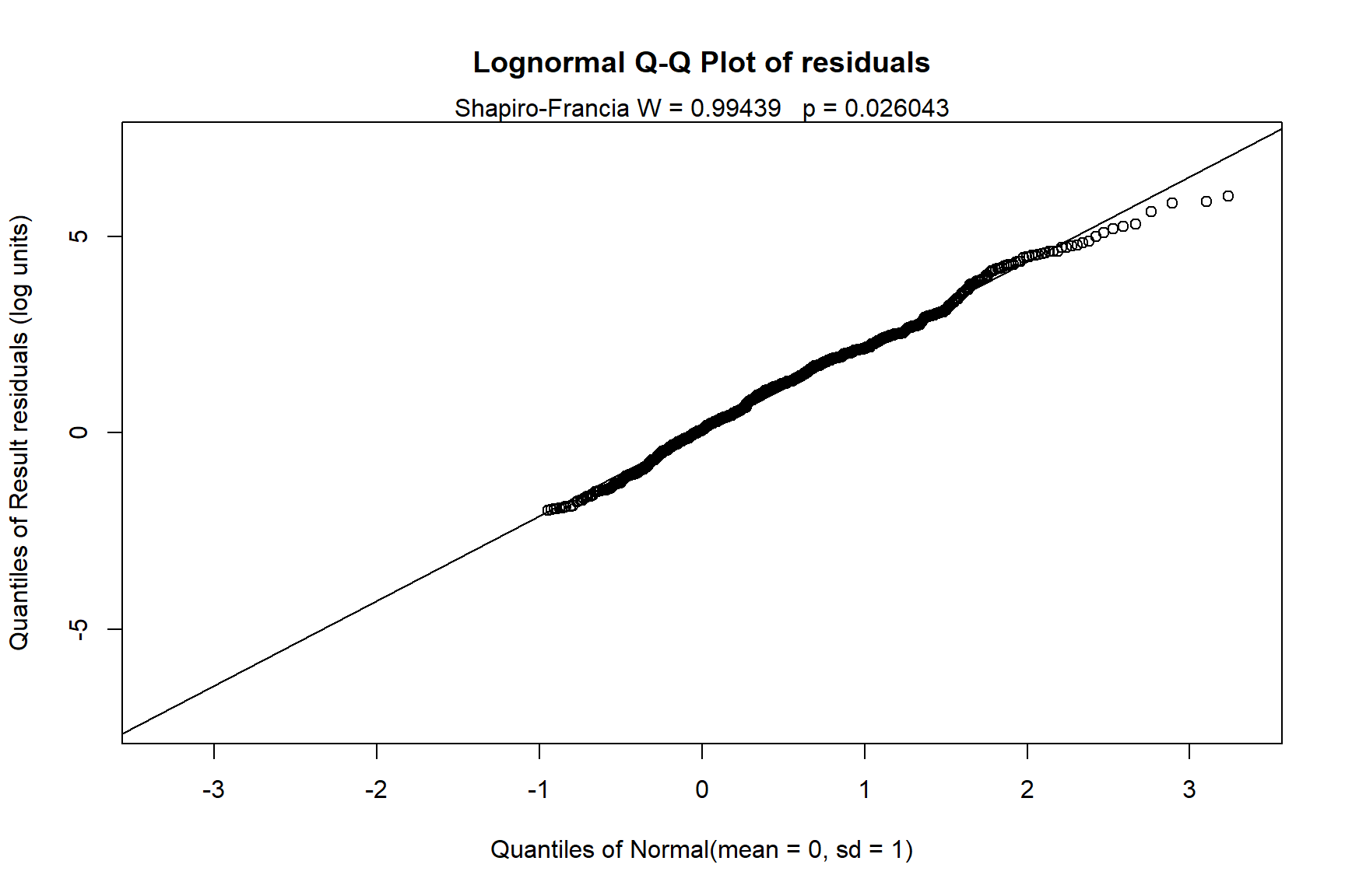
Let’s use the cenQQ() function in the NADA2 package to plot a censored quantile-quantile (Q-Q) plot for the bifenthrin data assuming a lognormal distribution.
# Plot a quantile-quantile (Q-Q) plot
with(bif,
  cenQQ(
    x.var = Result,
    cens.var = Censored,
    dist = 'lnorm',
    Yname = 'bifenthrin'
  )
)
It appears that the data deviate from a lognormal distribution in the tails.
Descriptive Statistics
Let’s calculate descriptive statistics using rROS, MLE, and KM methods.
# Get descriptive statistics using rROS, MLE, and K-M methods
with(bif, censtats(obs = Result, censored = Censored)) %>%
  kbl() %>%
  kable_minimal(full_width = F, position = "left")
##           n       n.cen     pct.cen
## 11155.00000  8183.00000    73.35724
| median | mean | sd | |
|---|---|---|---|
| K-M | NA | 0.0163454 | 0.1188787 |
| ROS | 0.0004277 | 0.0162992 | 0.1188229 |
| MLE | 0.0003508 | 0.0409129 | 4.7714440 |
Let’s plot the rROS model for the bifenthrin data.
# Robust regression on order statistics (rROS)
bif.ros <- with(bif,
  cenros(
    obs = Result,
    censored = Censored,
    forwardT = 'log', reverseT = 'exp'
  )
)
plot(bif.ros)
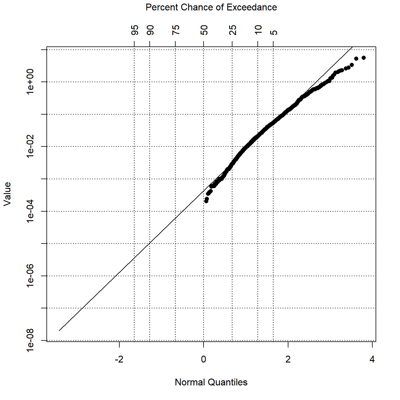
From the probability plot, it looks like the data do not reasonable fit a lognormal distribution.
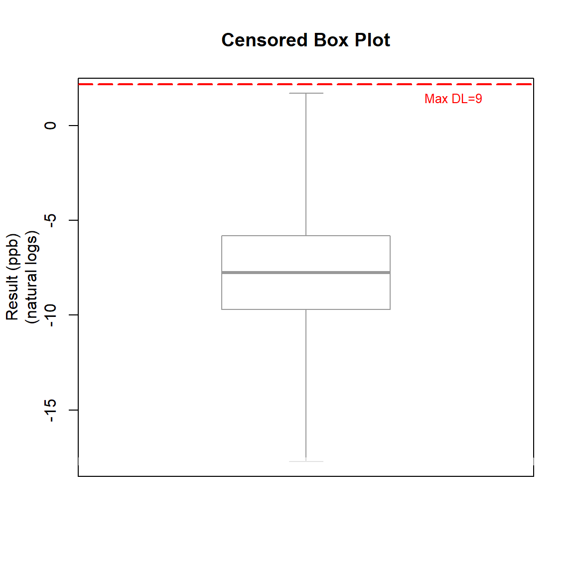
Let’s create a censored box plot of the bifenthrin data using the NADA2 package.
# Create censored boxplot using NADA2 package
with(bif,
  cboxplot(
    x1 = Result, x2 = Censored,
    LOG = TRUE,
    show = TRUE,
    Ylab = 'Result (ppb)',
    Xlab = NA,
    Title = 'Censored Box Plot',
    minmax = TRUE,
    printstat = FALSE
  )
)
Upper Limits
Let’s using the EnvStats package to estimate the 95% upper confidence limit (UCL) on the mean bifenthrin concentration nonparametrically.
# Estimate 95% UCL nonparametrically
set.seed(1)
ucls <- with(bif,
  enparCensored(
    x = Result,censored = Censored,
    ci = TRUE, ci.method = 'bootstrap',
    ci.type = 'upper', conf.level = 0.95,
    n.bootstraps = 1000
  )
)
The percentile bootstrap 95% UCL is 0.0182 ppb and the bias-corrected accelerated (BCa) bootstrap 95% UCL is 0.0181 ppb. Singh et al. (2006) suggest using the BCa UCL estimate for up to 40% non-detects and the percentile bootstrap for greater than 40% non-detects.
Let’s compute a 95/95 upper tolerance limit (UTL95-95) using the NADA2 package.
# Compute UTL95-95 using EnvStats
with(bif,
  cenTolInt(
    x.var = Result,
    cens.var = Censored,
    conf = 0.95,
    cover = 0.95,
    method.fit = 'rROS'
  )
) %>%
  kbl() %>%
  kable_minimal(full_width = F, position = "left")
| Distribution | 95th Pctl | 95% UTL | BIC | Method |
|---|---|---|---|---|
| Lognormal | 0.0512534 | 0.0549626 | -4057.037 | rROS |
| Gamma | 0.0739547 | 0.0778294 | -3480.892 | rROS |
| Normal | 0.1986751 | 0.2044418 | 76959.974 | rROS |
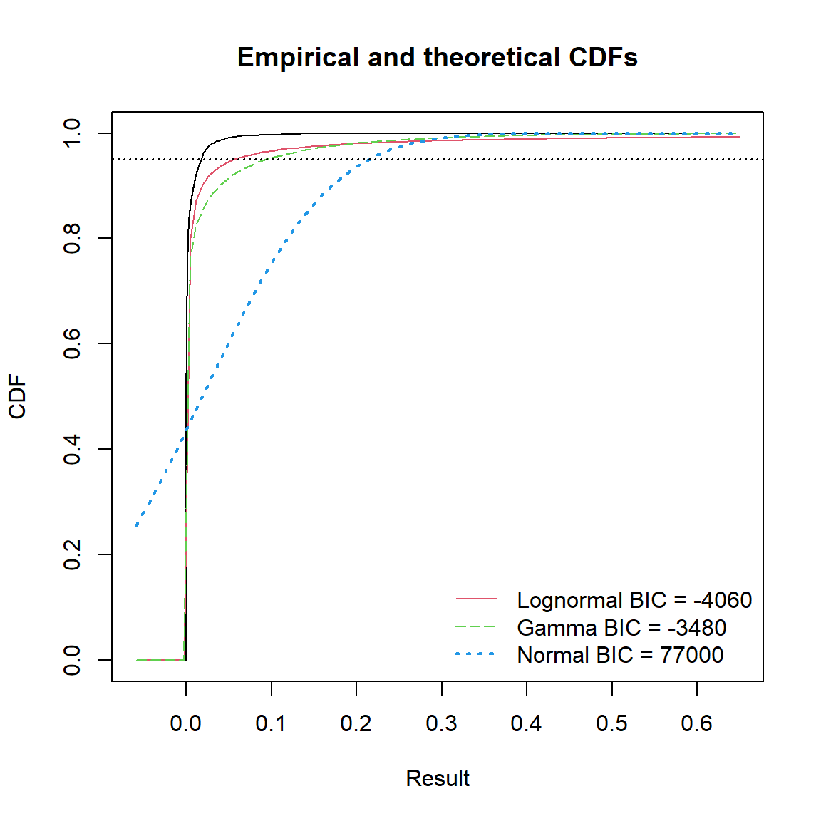
Based on the provided Bayesian information criterion (BIC), a lognormal distribution provides the best fit to the data. The UTL95-95 for a lognormal distribution is 0.0550 ppb.
Let’s compute a 95/95 upper tolerance limit (UTL95-95) using a code that I developed.
# Compute UTL95-95 using custom code
source('functions/get_utls.R')
utls <- get_utls(
  dd = bif, method = 'rROS',
  cover = 0.95, alpha = 0.05,
  trans = TRUE
)
utls %>%
  kbl() %>%
  kable_minimal(full_width = F, position = "left")
| bifenthrin | |
|---|---|
| METHOD | rROS |
| COVERAGE | 0.95 |
| ALPHA | 0.05 |
| UTL.NORM | 0.2044418 |
| UTL.GAMMA.WH | 0.07782936 |
| UTL.GAMMA.HW | 0.07054979 |
| UTL.LNORM | 0.05496264 |
| UTL.NP | 0.0651 |
| DIST | Nonparametric |
| UTL | 0.0651 |
A nonparametric UTL95-95 is recommended. The nonparametric UTL95-95 is 0.0651 ppb.
Compare Groups
Let’s create censored box plots for bifenthrin concentrations by sample type.
# Create censored boxplot by sample type using NADA2 package
with(bif,
  cboxplot(
    x1 = Result, x2 = Censored,
    xgroup = SampleType,
    LOG = TRUE,
    show = TRUE,
    Ylab = 'Result (ppb)',
    Xlab = 'Sample Type',
    Title = 'Censored Box Plot',
    minmax = TRUE,
    printstat = FALSE
  )
)
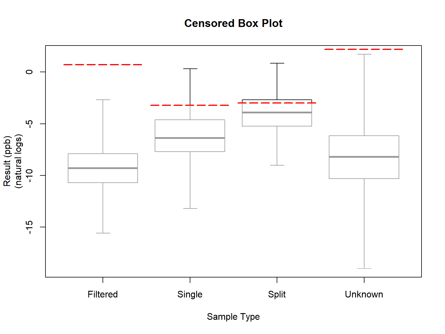
Let’s perform a nonparametric Peto-Peto test of differences in cumulative distribution functions (cdfs) between sample types The test is followed by a nonparametric multiple comparison test using the Benjamini-Hochberg (BH) method for adjusting p-values.
# Perform nonparametric test of differences in cdfs between groups
with(bif,
  cen1way(
    x1 = Result, x2 = Censored,
    group = SampleType,
    mcomp.method = 'BH'
  )
)
##          grp      N   PctND     KMmean       KMsd   KMmedian
## 1   Filtered   1927   97.61   0.001124   0.003126     <7e-04
## 2     Single   2658   50.30   0.015300   0.055030    0.00155
## 3      Split    183   78.14   0.135600   0.268800      <0.05
## 4    Unknown   6387   75.50   0.018910   0.144400     <1e-04
##
##       Oneway Peto-Peto test of CensData: Result   by Factor: SampleType
##       Chisq = 1049   on 3 degrees of freedom     p = 3.43e-227
##
## 	Pairwise comparisons using Peto & Peto test
##
## data:  CensData and Factor
##
##         Filtered Single  Split
## Single  < 2e-16  -       -
## Split   < 2e-16  4.2e-16 -
## Unknown < 2e-16  < 2e-16 < 2e-16
##
## P value adjustment method: BH
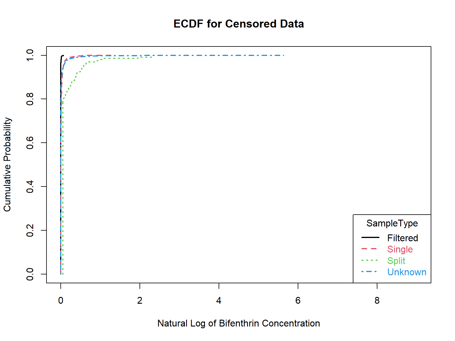
Let’s plot censored empirical cumulative distribution functions (ecdfs) of bifenthrin concentrations for each sample type. This graphically illustrates the differences between the data groups as was done using the Peto-Peto test.
with(bif,
  cen_ecdf(
    x.var = Result,
    cens.var = Censored,
    xgroup = SampleType,
    Ylab = 'Natural Log of Bifenthrin Concentration'
  )
)
Trend Analysis: Placer County
Let’s perform censored regression using MLE for bifenthrin concentrations in Placer county.
# MLE censored regression for bifenthrin concentrations in the Placer county
with(bif[bif$County == 'Placer',],
  cencorreg(
    y.var = Result, cen.var = Censored,
    x.vars = Date,
    LOG = TRUE, verbose = 2
  )
)
##  Likelihood R = -0.4254                     AIC = 977.823
## Rescaled Likelihood R = -0.4315            BIC = 987.8119
##  McFaddens R = -0.2361
##
## Call:
## survreg(formula = "log(Result)", data = "Date", dist = "gaussian")
##
## Coefficients:
## (Intercept)        Date
## 417.0804887  -0.2095288
##
## Scale= 1.665824
##
## Loglik(model)= -485.4   Loglik(intercept only)= -514.1
## 	Chisq= 57.31 on 1 degrees of freedom, p= 3.73e-14
## n= 287
Let’s perform nonparametric censored regression using the Akritas-Theil-Sen (ATS) method for bifenthrin concentrations in Placer county.
# Akritas-Theil-Sen regression for bifenthrin concentrations in the Placer county
with(bif[bif$County == 'Placer',],
  ATS(
    y.var = Result, y.cen = Censored,
    x.var = Date,
    LOG = TRUE
  )
)
## Akritas-Theil-Sen line for censored data
##
## ln(Result) = 405.5427 -0.2035 * Date
## Kendall's tau = -0.2784   p-value = 0
##
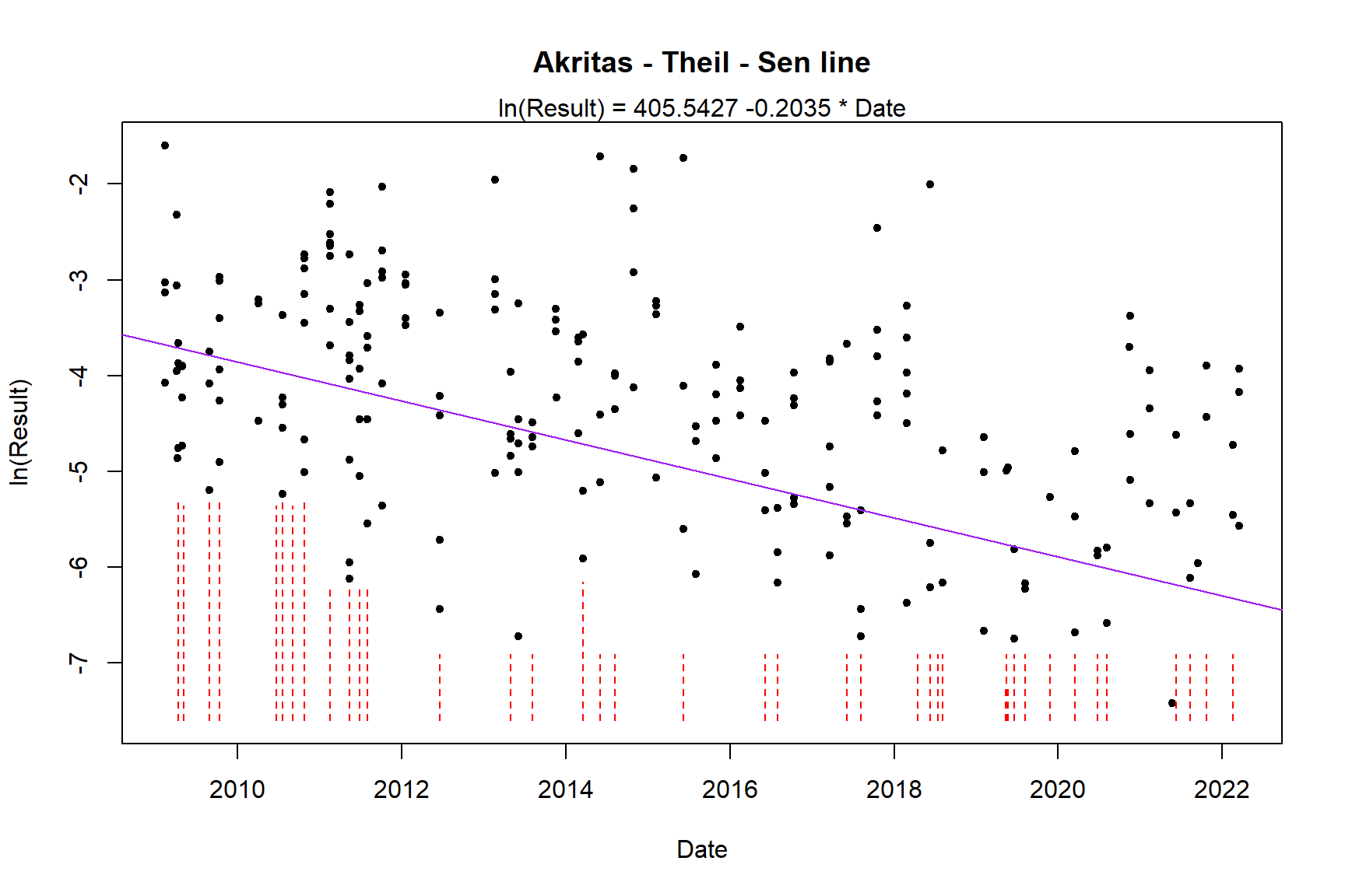
Both MLE and ATS indicate a decreasing trend in bifenthrin concentrations in Placer county.
Trend Analysis: Orange County
Let’s perform censored regression using MLE for bifenthrin concentrations in Orange county.
# MLE censored regression for bifenthrin concentrations in the Orange county
with(bif[bif$County == 'Orange',],
  cencorreg(
    y.var = Result, cen.var = Censored,
    x.vars = Date,
    LOG = TRUE, verbose = 2
  )
)
##  Likelihood R = 0.03358                     AIC = 3469.832
## Rescaled Likelihood R = 0.03421            BIC = 3483.684
##  McFaddens R = 0.01843
##
## Call:
## survreg(formula = "log(Result)", data = "Date", dist = "gaussian")
##
## Coefficients:
##  (Intercept)         Date
## -34.12532850   0.01446953
##
## Scale= 2.21632
##
## Loglik(model)= -1731.4   Loglik(intercept only)= -1732
## 	Chisq= 1.18 on 1 degrees of freedom, p= 0.278
## n= 1043
Let’s perform nonparametric censored regression using the ATS method for bifenthrin concentrations in Orange county.
# Akritas-Theil-Sen regression for bifenthrin concentrations in the Orange county
with(bif[bif$County == 'Orange',],
  ATS(
    y.var = Result, y.cen = Censored,
    x.var = Date,
    LOG = TRUE
  )
)
## Akritas-Theil-Sen line for censored data
##
## ln(Result) = -112.091 + 0.053 * Date
## Kendall's tau = 0.0642   p-value = 0.00184
##
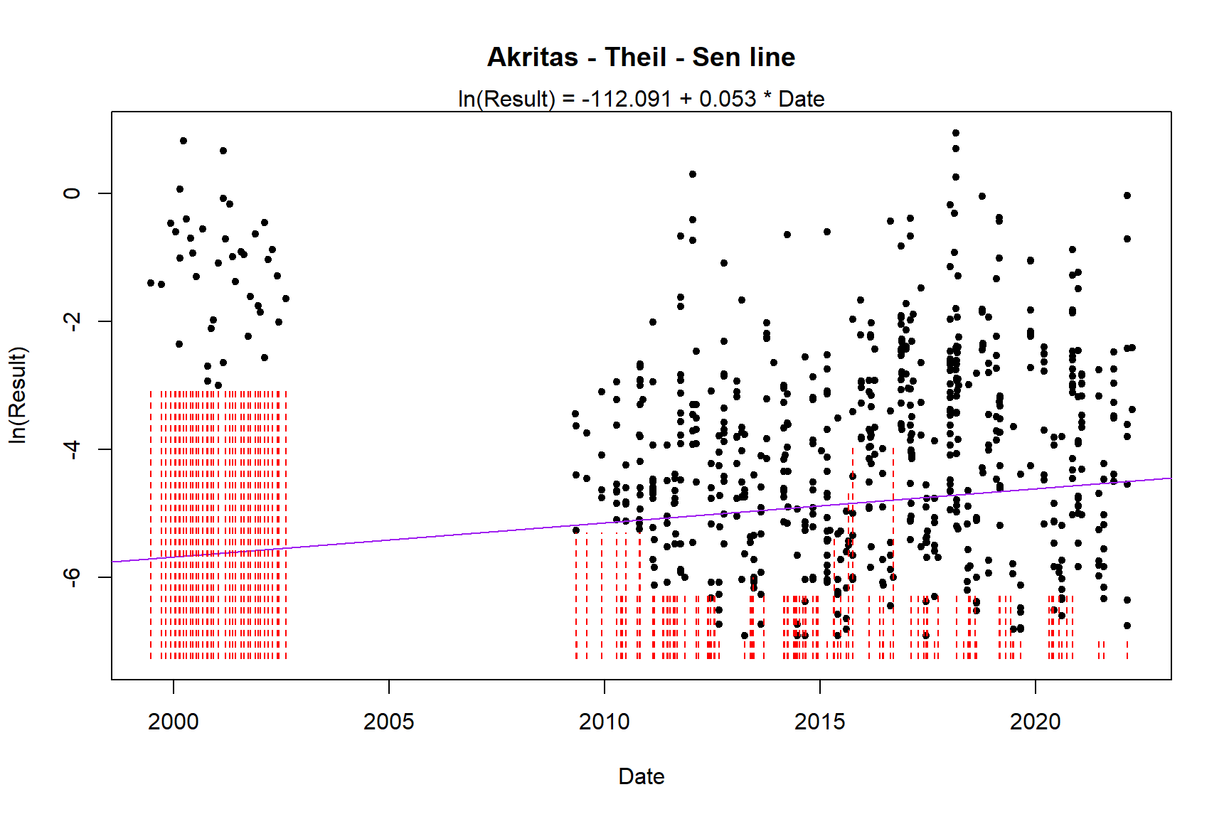
Both MLE and ATS indicate an increasing trend in bifenthrin concentrations in Orange county.
Trend Analysis: Median State-Wide Concentration
Let’s perform nonparametric censored regression using the ATS method for the annual state-wide median bifenthrin concentrations.
# Get median bifenthrin concentration by year
bif_med <- bif %>%
  group_by(Year) %>%
  summarize(
    Obs = length(Result),
    Dets = length(Result[Detected == 'Y']),
    Result = median(Result),
    Detected = ifelse(Dets == 0, 'N', 'Y'),
    Censored = ifelse(Dets == 0, TRUE, FALSE)
  ) %>%
  ungroup() %>%
  arrange(Year) %>%
  data.frame()

# Akritas-Theil-Sen regression for median bifenthrin concentrations
with(bif_med,
  ATS(
    y.var = Result, y.cen = Censored,
    x.var = Year,
    LOG = FALSE
  )
)
## Akritas-Theil-Sen line for censored data
##
## Result = 1.5286 -8e-04 * Year
## Kendall's tau = -0.6486   p-value = 1e-05
##
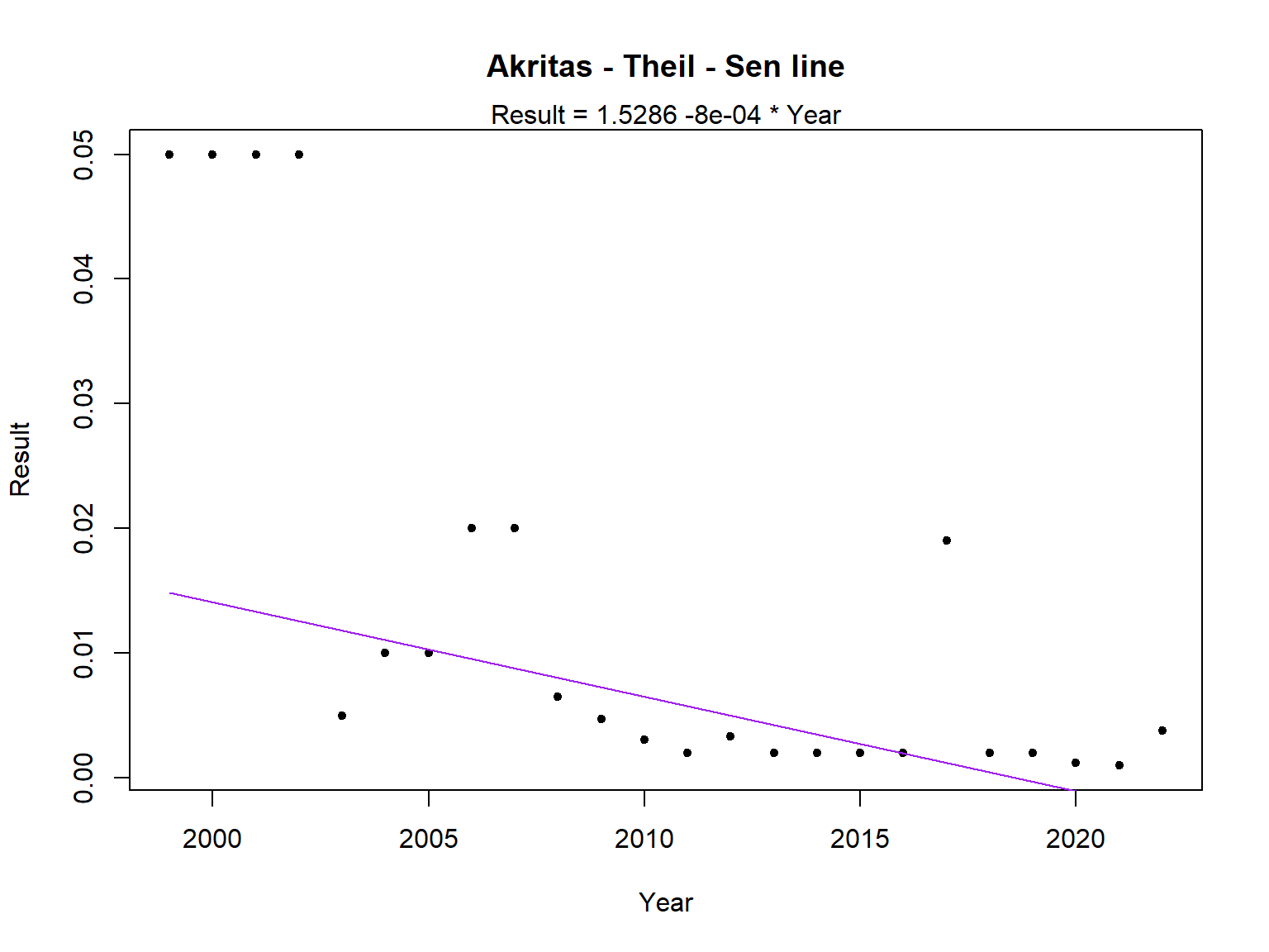
The annual state-wide median bifenthrin concentrations appear to be decreasing over time.
Mann-Kendall Trend Analysis: All Counties
Let’s perform Mann-Kendall (MK) trend analysis on the annual median bifenthrin concentrations for each county. The USEPA (2009) recommend that non-detects be included in the MK test by assigning them a common value that is less than the smallest measured value in the data set.
# Get median bifenthrin concentration by year for each county
bif_med_county <- bif %>%
  group_by(County, Year) %>%
  summarize(
    Chemical = 'Bifenthrin',
    Obs = length(Result),
    Dets = length(Result[Detected == 'Y']),
    Result = median(Result),
    DL = ifelse(Dets == 0, Result, NA),
    Units = 'ppb',
    Detected = ifelse(Dets == 0, 'N', 'Y'),
    Censored = ifelse(Dets == 0, TRUE, FALSE)
  ) %>%
  ungroup() %>%
  arrange(County, Year) %>%
  mutate(Date = as.POSIXct(paste0('1/1/', Year),format = '%m/%d/%Y')) %>%
  data.frame()

# Get Mann-Kendall trend trends
library(trendMK)

trends <- with(bif_med_county,
  trend(
    x = Result,
    detect = Detected,
    date = Date,
    loc = County,
    param = Chemical,
    censor_limit = DL,
    units_field = Units,
    flag_field = NA
  )
)

# Get number of statistically significant trends
all_trend <- length(trends$TREND)
inc_trend <- length(trends[trends$TREND == 'Increasing', ]$TREND)
dec_trend <- length(trends[trends$TREND == 'Decreasing', ]$TREND)

trend_counts <- paste(
  'The total cases evaluated with the Mann-Kendall test is', all_trend,
  ' \nThe total number of statistically significant trends is', inc_trend + dec_trend,
  ' \nThe number of increasing trends is', inc_trend,
  ' \nThe number of decreasing trends is', dec_trend, '\n'
)
cat(trend_counts)
## The total cases evaluated with the Mann-Kendall test is 53
## The total number of statistically significant trends is 8
## The number of increasing trends is 6
## The number of decreasing trends is 2
The total cases evaluated with the MK test is 53. The total number of statistically significant trends is 8. The number of increasing trends is 6. The number of decreasing trends is 2.
Let’s graphically inspect the results of the MK test.
# Spread the trend results
trends_wide <- trends %>%
  dplyr::select(LOCID, PARAM, TREND) %>%
  spread(PARAM, TREND) %>%
  rename(County = LOCID)

# Function to create html color specs
get_spec <- function(x) {
  x = ifelse(x == 'Increasing', cell_spec(x, "html", color = "red", bold = T),
        ifelse(x == 'Decreasing', cell_spec(x, "html", color = "green", bold = T),
               cell_spec(x, "html", color = "black", bold = F)
        )
      )
  return(x)
}

# Assign colors by trend category
trends_sp <- trends_wide %>%
  mutate(across(.cols = everything(), get_spec))

# Create footnote
fn <- 'IS = insufficient data\n'

# Create table
trends_sp %>%
  kable('html', escape = F, align = 'c') %>%
  kable_classic(full_width = F, font_size = 12, html_font = 'Cambria') %>%
  kableExtra::footnote(general = fn)
| County | Bifenthrin |
|---|---|
| Alameda | No Trend |
| Alpine | IS |
| Amador | IS |
| Butte | No Trend |
| Calaveras | IS |
| Colusa | No Trend |
| Contra Costa | No Trend |
| Del Norte | IS |
| El Dorado | IS |
| Estuary | No Trend |
| Fresno | No Trend |
| Glenn | No Trend |
| Humboldt | No Trend |
| Imperial | No Trend |
| Kern | No Trend |
| Kings | No Trend |
| Lake | No Trend |
| Los Angeles | Increasing |
| Madera | Increasing |
| Marin | No Trend |
| Mariposa | IS |
| Mendocino | IS |
| Merced | No Trend |
| Monterey | Increasing |
| Napa | IS |
| Ocean | IS |
| Orange | No Trend |
| Placer | Decreasing |
| Riverside | No Trend |
| Sacramento | No Trend |
| San Benito | IS |
| San Bernardino | No Trend |
| San Diego | No Trend |
| San Francisco | IS |
| San Joaquin | Increasing |
| San Luis Obispo | No Trend |
| San Mateo | No Trend |
| Santa Barbara | No Trend |
| Santa Clara | Decreasing |
| Santa Cruz | No Trend |
| Shasta | No Trend |
| Siskiyou | IS |
| Solano | No Trend |
| Sonoma | No Trend |
| Stanislaus | No Trend |
| Sutter | Increasing |
| Tehama | IS |
| Trinity | IS |
| Tulare | No Trend |
| Tuolumne | IS |
| Ventura | No Trend |
| Yolo | Increasing |
| Yuba | No Trend |
| Note: | |
|
IS = insufficient data |
Let’s inspect the samples where the MK test indicates either an increasing or decreasing trend.
# Inspect samples where trends are either increasing or decreasing
trends %>%
  filter(TREND %in% c('Increasing', 'Decreasing')) %>%
  dplyr::select(LOCID, COUNT, S, PVAL, SLOPE, RESULT, TREND) %>%
  rename(COUNTY = LOCID) %>%
  mutate(
    S = as.numeric(S),
    PVAL = round(as.numeric(PVAL), 3),
    SLOPE = round(as.numeric(SLOPE), 5)
  ) %>%
  arrange(TREND, COUNTY) %>%
  kbl() %>%
  kable_minimal(full_width = F, position = "left")
| COUNTY | COUNT | S | PVAL | SLOPE | RESULT | TREND |
|---|---|---|---|---|---|---|
| Placer | 14 | -53 | 0.002 | -0.00138 | 99.8% (sig -) | Decreasing |
| Santa Clara | 11 | -29 | 0.013 | -0.00042 | 98.7% (sig -) | Decreasing |
| Los Angeles | 15 | 71 | 0.000 | 0.00032 | 100% (sig +) | Increasing |
| Madera | 9 | 21 | 0.017 | 0.00004 | 98.3% (sig +) | Increasing |
| Monterey | 16 | 61 | 0.002 | 0.00043 | 99.8% (sig +) | Increasing |
| San Joaquin | 20 | 84 | 0.003 | 0.00003 | 99.7% (sig +) | Increasing |
| Sutter | 13 | 40 | 0.007 | 0.00003 | 99.3% (sig +) | Increasing |
| Yolo | 18 | 47 | 0.041 | 0.00000 | 95.9% (sig +) | Increasing |
ATS Trend Analysis: All Counties
Replacing non-detects by a common value that is less than the smallest detected value is an imperfect remedy for trend testing. An alternative approach is to use the ATS method for trend testing. The significance test for the ATS slope is the same test as that for Kendall’s tau correlation (Helsel 2012). When the explanatory variable is a measure of time, the significance test for the slope is a test for (temporal) trend.
Let’s perform ATS trend analysis on the annual median bifenthrin concentrations for each county and compare the results to the MK trend test.
# Get ATS trend trends
ats_trends <- with(bif_med_county,
  trendATS(
    x = Result,
    detect = Detected,
    date = Date,
    loc = County,
    param = Chemical,
    censor_limit = DL,
    units_field = Units,
    flag_field = NA
  )
)

# Inspect difference between Mann-Kendall test results and ATS test results
trend_diff <- trends %>%
  filter(S != 'IS') %>%
  droplevels() %>%
  mutate(
    S = as.numeric(S),
    PVAL = round(as.numeric(PVAL), 3)
  ) %>%
  dplyr::select(LOCID, COUNT, DET, S, PVAL, TREND) %>%
  rename(
    MK.S = S,
    MK.PVAL = PVAL,
    MK.TREND = TREND
  ) %>%
  right_join(
    ats_trends %>%
      filter(S != 'IS') %>%
      droplevels() %>%
      mutate(
        S = as.numeric(S),
        PVAL = round(as.numeric(PVAL), 3)
      ) %>%
      dplyr::select(LOCID, S, PVAL, TREND) %>%
      rename(
        ATS.S = S,
        ATS.PVAL = PVAL,
        ATS.TREND = TREND
      ),
    by = 'LOCID'
  ) %>%
  rename(COUNTY = LOCID) %>%
  filter(MK.TREND != ATS.TREND)

# Inspect difference
trend_diff %>%
  kbl() %>%
  kable_minimal(full_width = F, position = "left")
| COUNTY | COUNT | DET | MK.S | MK.PVAL | MK.TREND | ATS.S | ATS.PVAL | ATS.TREND |
|---|---|---|---|---|---|---|---|---|
| Madera | 9 | 3 | 21 | 0.017 | Increasing | 6 | 0.306 | No Trend |
| San Joaquin | 20 | 8 | 84 | 0.003 | Increasing | 0 | 0.513 | No Trend |
| Sutter | 13 | 4 | 40 | 0.007 | Increasing | 6 | 0.383 | No Trend |
| Yolo | 18 | 6 | 47 | 0.041 | Increasing | -1 | 0.500 | No Trend |
There are four counties where the MK test indicates an increasing trend in concentration but the ATS test indicates a nonsignificant test result (i.e., the null hypothesis of no trend cannot be rejected at the stated significance level). The p-values between the two test methods are significantly different for these four counties.
Conclusions
Environmental data are frequently left-censored, indicating that some values are less than the limit of quantification for the analytical methods employed. These data are problematic because censored (non-detect) values are known only to range between zero and the censoring limit. This complicates analysis of the data, including estimating statistical parameters, characterizing data distributions, and conducting inferential statistics. This post has demonstrated various procedures and methods that are available in R for analyzing data containing a mixture of detects and non-detects. These methods make few or no assumptions about the data, or substitute arbitrary values (e.g., one-half the detection or reporting limit) for the non-detects.
References
Helsel, D.R. 2012. Statistics for Censored Environmental Data Using Minitab and R, Second Edition. John Wiley and Sons, NJ.
Kaplan, E.L. and O. Meier. 1958. Nonparametric Estimation from Incomplete Observations. JASA 53, 457-481.
Millard, S.P. 2013. EnvStats: An R Package for Environmental Statistics. Springer, NY.
Shapiro, S. S. and M. B. Wilk. 1965. An analysis of variance test for normality (complete samples). Biometrika, 52, 591-611.
Singh, A., R. Maichle, and S. Lee. 2006. On the Computation of a 95% Upper Confidence Limit of the Unknown Population Mean Based Upon Data Sets with Below Detection Limit Observations. EPA/600/R-06/022. Office of Research and Development, U.S. Environmental Protection Agency. March.
United States Environmental Protection Agency (USEPA). 2009. Statistical Analysis of Groundwater Monitoring Data at RCRA Facilities: Unified Guidance. EPA-530-R-09-007. Office of Resource Conservation and Recovery, U.S. Environmental Protection Agency. March.
Wilcox, R and R. 2010. Fundamentals of Modern Statistical Methods, Second Edition. Springer, NY.
- Posted on:
- September 16, 2023
- Length:
- 40 minute read, 8410 words
- See Also: