Introduction

Drought is a part of normal climate variability in many climate zones. Althought drought is commonly considered a deficiency in precipitation over an extended period, it is more complex than simple precipitation deficits. Drought can develop quickly and last only for a matter of weeks, exacerbated by extreme heat and/or wind, but more commonly drought can persist for months or years. Factors affecting drought intensity include temporal and spatial variability of precipitation events, rainfall intensity, and temperature and cloud cover which influence evaporation. Drought causes losses to agriculture; affects domestic water supply, energy production, public health, and wildlife; and contributes to wildfire, to name a few of its effects.

The U.S. Drought Monitor (USDM) is a map that is updated each Thursday to show the location and intensity of drought across the country. The USDM is a collaborative effort between a number of federal agencies including NOAA/NWS, U.S. Department of Agriculture, and the National Drought Mitigation Center. The USDM rates the severity of drought across the United States, including Puerto Rico and and Affiliated Pacific Islands, based on numerous meteorological and hydrological observations, environmental indices, impacts, and knowledge from local experts. The NDMC, based at the University of Nebraska in Lincoln, leads the coordination of the weekly drought monitor process and provides the maps, data, and statistics to the public.

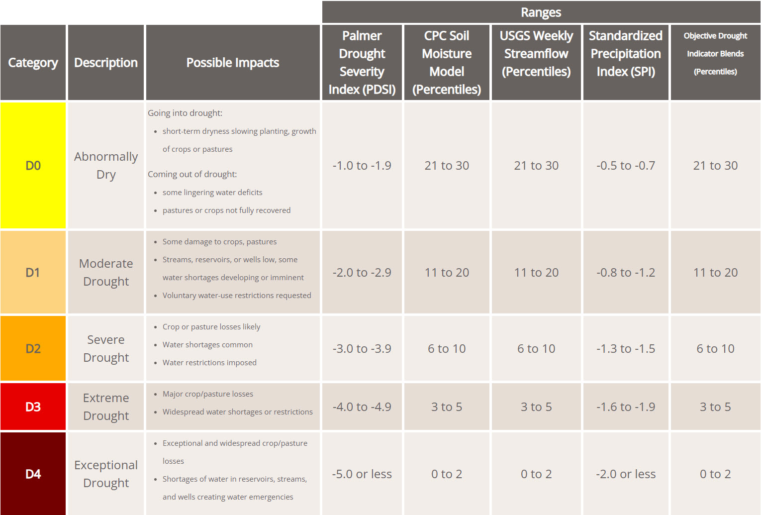
The USDM uses a five-category system for drought intensity. These categories are: Abnormally Dry or D0, (a precursor to drought, but not actually drought), Moderate (D1), Severe (D2), Extreme (D3), and Exceptional (D4) Drought. These USDM severity categories and commonly associated impacts are shown below in the table.

The USDM provides an API to download data for all USDM categories for each week of the selected time period and location. Data options include percent of area, total area, percent of population and total population. Spatial scale choices include national, state, county, and urban areas. Using these data and the R statistical programming language, we can visualize drought severity across the United States for various time periods as static maps or even as an animated map.

Data

Data containing drought category and the percent of population affected by each category were downloaded from the USDM. The downloaded data include values between January 1, 2019 and July 7, 2022; however, additional data are available at the USDM. Let’s read the comma-delimited file containing the data.

# Read data in comma-delimited file
dat <- read.csv('data/dm_export_20190101_20220707.csv', header = T)

Now that the data are loaded, let’s prep the data for analysis. Let’s convert the data from wide to long format, use the R package janitor to clean the variable names, and create the drought category levels. Let’s then use the group_by() and slice_max() functions to select the highest drought level for each week (valid_start) and each county (fips) from the 5 levels (None, D1, D2, D3, D4) based on percent of population affected.

Note that we are filtering the data to only include the first results in January 2019 and 2022. This significantly reduces computational time and memory requirements when creating static maps for a select number of dates. However, filtering on dates should not be performed if creating an animated map.

# Prep data
us_drought <- dat %>%
    filter(
    ValidStart %in% c('2019-01-01', '2022-01-04')  # remove for animation
  ) %>%
  pivot_longer(
    cols = c(None:D4), names_to = 'drought_lvl' , values_to = 'pct_pop'
  ) %>%
  janitor::clean_names() %>%
  mutate(fips = sprintf('%05d', fips)) %>%
  mutate(
    drought_lvl = factor(
      drought_lvl, 
      levels = c('None' , 'D0' , 'D1' , 'D2' , 'D3' , 'D4'),
      labels = c('None', 'Abnormal', 'Moderate', 'Severe', 'Extreme', 'Exceptional')
    )
  ) %>%
  group_by(valid_start, fips) %>%
  slice_max(order_by = pct_pop, n = 1) %>%
  ungroup()

Now, let’s import state and counties shapefiles using the R package tigris. The tigris package allows users to directly download and use TIGER/Line shapefiles from the US Census Bureau. Let’s focus our analysis on the continental United States that includes the 48 contiguous states but not Alaska, Hawaii, Puerto Rico, and the other U.S. territories. We can use the U.S. Federal Information Processing Standard Publication (FIPS) state codes for Alaska, Hawaii, and Puerto Rico to remove those states from the downloaded shapefile. The FIPS codes for Alaska, Hawaii, Puerto Rico are ‘02’, ‘15’, and ‘72.’

Let’s use the st_simplify() function from the R package sf to simplify the polygons in the counties shapefile to a lower definition. The st_simplify() function uses the GEOS implementation of the Douglas-Peucker algorithm to reduce the vertex count. st_simplify() uses the dTolerance parameter to control the level of generalization in map units (see Douglas and Peucker 1973 for details). This will reduce memory requirements.

counties <- counties(progress_bar = FALSE) %>%
  dplyr::select(
    state_id = STATEFP,
    county_id = GEOID,
    county_name = NAMELSAD
  ) %>%
  rename(fips = county_id) %>%
  dplyr::filter(!(state_id %in% c('02', '15', '72'))) %>%
  st_simplify(dTolerance = 1)

Let’s join the USDM data with the spatial data for mapping purposes. We will define the join based on the common attribute field, which is the FIPS county code.

# Join into one table of geoinfo and drought categories
doParallel::registerDoParallel()
counties_drought <- counties %>% 
  inner_join(us_drought, by = 'fips')

Maps

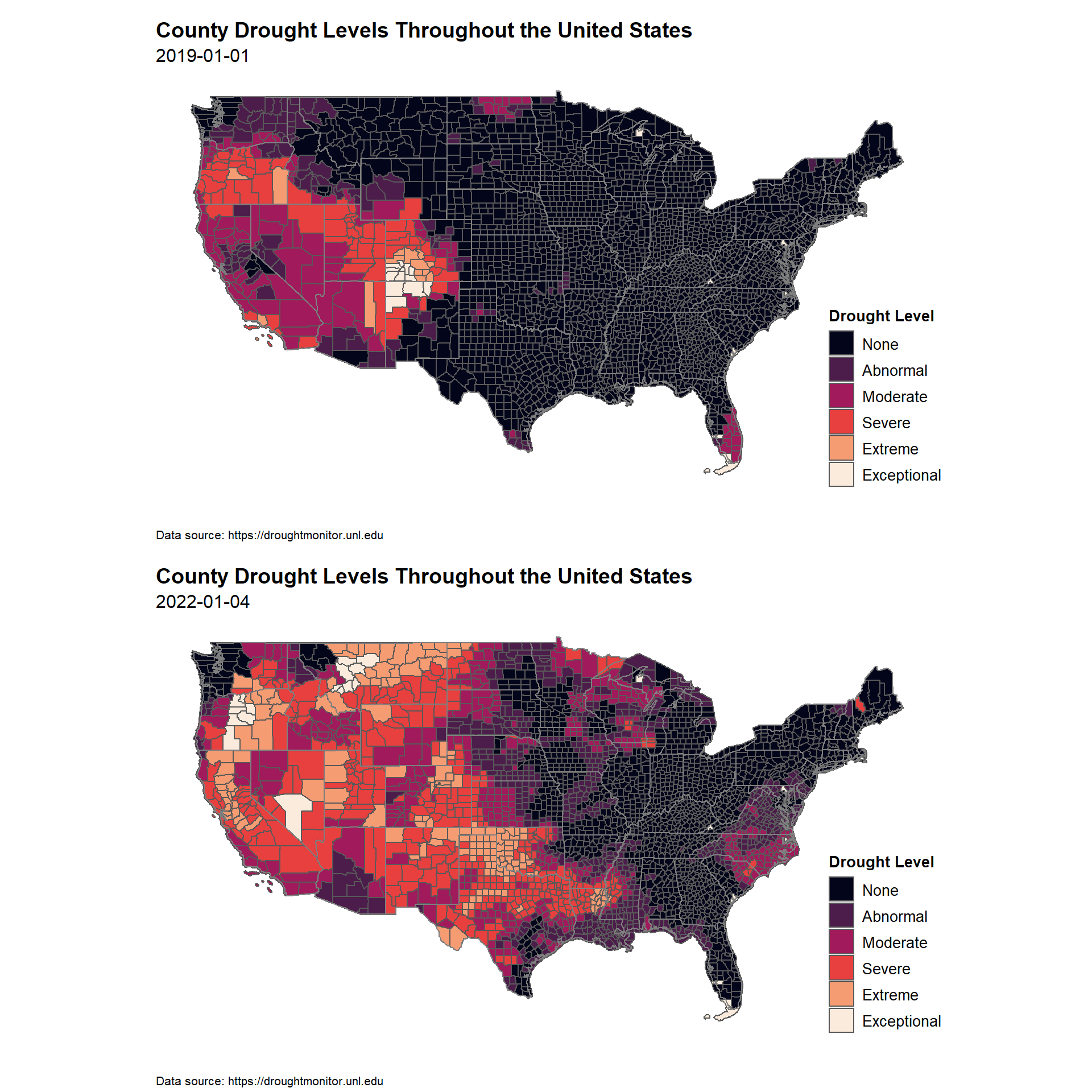
Now, let’s use the R package ggplot2 to create static maps showing the USDM severity categories based on percent of population affected for the two time periods.

# Get min and max dates
min_date <- min(counties_drought$valid_start)
max_date <- max(counties_drought$valid_start)

# Create first plot using min date
p1 <- counties_drought %>%
  filter(valid_start == min_date) %>%
  ggplot(aes(fill = drought_lvl)) +
  geom_sf() +
  borders('state') +
  scale_fill_viridis_d(option = 'rocket', begin = 0, end = 1) +
  labs(
    title = 'County Drought Levels Throughout the United States',
    subtitle = min_date,
    caption = 'Data source: https://droughtmonitor.unl.edu',
    fill = 'Drought Level'
  ) +
  coord_sf() +
  ggthemes::theme_map() +
  theme(
    plot.title = element_text(size = 14 , face = 'bold'),
    plot.subtitle = element_text(size = 12),
    plot.caption = element_text(vjust = -10, hjust = 0, size = 8),
    legend.title = element_text(size = 10, face = 'bold'),
    legend.text = element_text(size = 10),
    legend.position = c(0.85, 0),
    plot.margin = margin(0.5, 0.5, 0.7, 0.5, unit = 'cm')
  )

# Create second plot using max date
p2 <- counties_drought %>%
  filter(valid_start == max_date) %>%
  ggplot(aes(fill = drought_lvl)) +
  geom_sf() +
  borders('state') +
  scale_fill_viridis_d(option = 'rocket', begin = 0, end = 1) +
  labs(
    title = 'County Drought Levels Throughout the United States',
    subtitle = max_date,
    caption = 'Data source: https://droughtmonitor.unl.edu',
    fill = 'Drought Level'
  ) +
  coord_sf() +
  ggthemes::theme_map() +
  theme(
    plot.title = element_text(size = 14 , face = 'bold'),
    plot.subtitle = element_text(size = 12),
    plot.caption = element_text(vjust = -10, hjust = 0, size = 8),
    legend.title = element_text(size = 10, face = 'bold'),
    legend.text = element_text(size = 10),
    legend.position = c(0.85, 0),
    plot.margin = margin(0.5, 0.5, 0.7, 0.5, unit = 'cm')
  )

grid.arrange(p1, p2, ncol = 1)

An animated map can be created using the R package gganimate and the code snippet shown below. Recall that we filtered the USDM data to only include the first results in January 2019 and 2022. If creating an animated map, the USDM data will need to be prepped with this filter removed. Because the data contain over one-half a million records, computation time and memory requirements will significantly increase, especially when joining the USDM data with the spatial data.

# Load libraries
library(gganimate)
library(gifski)

drought_map <- counties_drought %>%
#  filter(valid_start >= '2022-01-01') %>% # for testing purposes
  ggplot(aes(fill = drought_lvl)) +
  geom_sf() +
  borders('state') +
  transition_manual(valid_start) +
  scale_fill_viridis_d(option = 'rocket', begin = 0, end = 1) +
  labs(
    title = 'County Drought Levels Over Time Throughout the United States',
    subtitle = '{current_frame}',
    caption = 'Data source: https://droughtmonitor.unl.edu',
    fill = 'Drought Level'
  ) +
  ggthemes::theme_map() +
  coord_sf() +
  theme(
    plot.title = element_text(size = 50 , face = 'bold'),
    plot.subtitle = element_text(vjust = -1, size = 50),
    plot.caption = element_text(size = 30),
    legend.title = element_text(size = 36, face = 'bold'),
    legend.text = element_text(size = 36),
    legend.key.height = unit(2.5, 'line'),
    legend.position = c(0, 0.05),
    plot.margin = margin(0, 0.5, 1, 0.5, unit = 'cm')
  )

drought_map %>%
animate(
  fps = 55, nframe = 300, 
  height = 2000, width = 2340,
  start_pause = 1, end_pause = 1,
  renderer = gifski_renderer('us_drought.gif')
)

The USDM gives a broad overview of drought conditions in the United States. Although it is based on many types of data, it is not intended to replace local information that might describe conditions more precisely for a particular region. The USDM is used to trigger aid to farmers and to help officials such as local water resource managers make recommendations for conserving water. Because drought happens incrementally, its effects can be underestimated. Vulnerability is not captured in the USDM. Because frequent, pervasive droughts are becoming more common, a moderate dry period may now produce more serious effects than it would have in the past.