Introduction

Dimensionality reduction comprises a number of approaches that turn a set of (potentially many) variables into a smaller number of variables that retain as much of the original, multidimensional information as possible. Reducing data dimensionality down to two or three, makes it possible to visualize the data on a 2D or 3D plot. Important insights can be gained by analysing patterns in the simplified data, such as whether clusters are present in the data.

In this post, we will explore three powerful and popular dimensionality reduction algorithms: principal component analysis (PCA), t-distributed stochastic neighbor embedding (t-SNE), and uniform manifold approximation and projection (UMAP).

Data

Let’s use the oils data contained in the modeldata R package. These data represent samples of commercial edible vegetable oils. Gas chromatography was used to determine the fatty acid composition of each sample, namely palmitic, stearic, oleic, linoleic, linolenic, eicosanoic, and eicosenoic acids (Brodnjak-Voncina et al. 2005). Based on the fatty acid composition, the samples were placed into seven classes of oil.

# Load libraries
library(dplyr)
library(ggplot2)
library(cowplot)

# Load oils dataset from modeldata package
data(oils, package = 'modeldata')

str(oils)

## tibble [96 x 8] (S3: tbl_df/tbl/data.frame)
##  $ palmitic  : num [1:96] 9.7 11.1 11.5 10 12.2 9.8 10.5 10.5 11.5 10 ...
##  $ stearic   : num [1:96] 5.2 5 5.2 4.8 5 4.2 5 5 5.2 4.8 ...
##  $ oleic     : num [1:96] 31 32.9 35 30.4 31.1 43 31.8 31.8 35 30.4 ...
##  $ linoleic  : num [1:96] 52.7 49.8 47.2 53.5 50.5 39.2 51.3 51.3 47.2 53.5 ...
##  $ linolenic : num [1:96] 0.4 0.3 0.2 0.3 0.3 2.4 0.4 0.4 0.2 0.3 ...
##  $ eicosanoic: num [1:96] 0.4 0.4 0.4 0.4 0.4 0.4 0.4 0.4 0.4 0.4 ...
##  $ eicosenoic: num [1:96] 0.1 0.1 0.1 0.1 0.1 0.5 0.1 0.1 0.1 0.1 ...
##  $ class     : Factor w/ 7 levels "corn","olive",..: 4 4 4 4 4 4 4 4 4 4 ...

oils %>% count(class)

## # A tibble: 7 x 2
##   class         n
##   <fct>     <int>
## 1 corn          2
## 2 olive         7
## 3 peanut        3
## 4 pumpkin      37
## 5 rapeseed     10
## 6 soybean      11
## 7 sunflower    26

The data will be standardized by mean-centering and scaling to unit variance before conducting dimensionality reduction using the three methods.

Principal Component Analysis

One of the most widely used dimensionality reduction algorithms is PCA. PCA is used to reduce the dimensionality of a dataset with correlated variables by creating new uncorrelated variables (the principal components [PCs]) that are linear combinations of the data (Joliffe 1986). In PCA, eigenvalues represent the variance along a PC, and the eigenvector represents the direction of the principal axis through the original feature space. PCA will find as many principal axes as there are variables or one less than the number of cases in the dataset, whichever is smaller. The PCs are ordered such that the first few PCs account for most of the variation present in the original variables.

The built-in R function prcomp() can be used to perform PCA. When we view the pca object, we get a printout of some information of our model. The standard deviations component is a vector of the standard deviations of the data along each of the PCs. Because the variance is the square of the standard deviation, to convert these standard deviations into the eigenvalues for the PCs, we can simply square them. The rotation component contains the six eigenvectors. The eigenvectors describe how far along each original variable we go, so that we’re one unit along the principal axis away from the origin. These eigenvectors describe the direction of the principal axes.

# Perform PCA
oils_pca <- oils %>%
  dplyr::select(where(is.numeric)) %>% # select only the numeric variables
  tidyr::drop_na() %>% # to drop any NA
  scale() %>% # to initially normalise the variances
  prcomp() # to convert numeric data to principal components

# Inspect results
oils_pca

## Standard deviations (1, .., p=7):
## [1] 1.78631393 1.21432295 1.11849881 0.80775705 0.49010697 0.43543634 0.03437479
## 
## Rotation (n x k) = (7 x 7):
##                   PC1         PC2         PC3         PC4         PC5
## palmitic   -0.1724393 -0.69299469 -0.04593832  0.46972220 -0.19508286
## stearic    -0.4589668 -0.25101419 -0.24289349  0.18544207  0.61204669
## oleic       0.4578722 -0.39918199  0.14986398 -0.28962122  0.08386290
## linoleic   -0.4590266  0.44858975 -0.11564307  0.05114339 -0.07111895
## linolenic   0.3446082  0.27607934  0.23426894  0.80580939 -0.02884460
## eicosanoic  0.1682596 -0.01595516 -0.81991595  0.04591653 -0.46100031
## eicosenoic  0.4384013  0.14034544 -0.41942317  0.08389933  0.60157904
##                   PC6        PC7
## palmitic   -0.4661816 0.10904667
## stearic     0.5067647 0.03928963
## oleic       0.2409267 0.67792957
## linoleic   -0.2371904 0.71467174
## linolenic   0.2916300 0.12220735
## eicosanoic  0.2889776 0.03216008
## eicosenoic -0.4929535 0.01587562

If we pass our PCA results to the summary() function, we get a breakdown of the importance of each of the PCs.

summary(oils_pca)

## Importance of components:
##                           PC1    PC2    PC3     PC4     PC5     PC6     PC7
## Standard deviation     1.7863 1.2143 1.1185 0.80776 0.49011 0.43544 0.03437
## Proportion of Variance 0.4558 0.2107 0.1787 0.09321 0.03431 0.02709 0.00017
## Cumulative Proportion  0.4558 0.6665 0.8452 0.93843 0.97274 0.99983 1.00000

Now, let’s add the PCs to the original data.

# Add PCA results to data
oils2 <- cbind(oils, oils_pca$x)

t-Stochastic Neighborhood Embedding

When information in a set of variables cannot be extracted as a linear combination of the variables, nonlinear dimension-reduction algorithms can be utilized. One nonlinear dimension-reduction algorithm is t-SNE, developed by van der Maaten and Hinton (2008). t-SNE measures the distance between each observation in the dataset and every other observation, and then randomizes the observations across (usually) two new axes. The observations are then iteratively shuffled around these new axes until their distances to each other in this two-dimensional space are as similar to the distances in the original high-dimensional space as possible.

t-SNE is nonlinear because instead of finding new axes that are logical combinations of the original variables, it focuses on the similarities between nearby cases in a dataset and tries to reproduce these similarities in a lower-dimensional space. It can deal with more complex patterns of Gaussian clusters in multidimensional space compared to PCA. One of the downsides of this approach is that the axes are no longer interpretable, because they don’t represent logical combinations of the original variables.

We will use the tsne R package to perform t-SNE. Unlike PCA, t-SNE is a stochastic algorithm, so we need to set the seed to lock the random estimators for reproducibility.

# Load tSNE library
library(tsne)

# Run t-SNE
set.seed(1)
oils_tsne <- oils %>%
  dplyr::select(where(is.numeric)) %>%
  tidyr::drop_na() %>%
  scale() %>%
  tsne()

# Inspect results
str(oils_tsne)

##  num [1:96, 1:2] -19.27 -2.69 71.34 -22.25 76.38 ...

Now, let’s format the t-SNE results and add them to the original data.

# Format t-SNE results
oils_tsne <- oils_tsne %>%
  data.frame() %>%
  rename(
    tSNE1 = X1,
    tSNE2 = X2
  )

# Add t-SNE results to data
oils2 <- cbind(oils2, oils_tsne)

Uniform Manifold Approximation and Projection

UMAP is another nonlinear dimension-reduction algorithm that overcomes some of the limitations of t-SNE (McInnes et al. 2018). It works similarly to t-SNE in that it finds distances in a feature space with many variables and then tries to reproduce these distances in low-dimensional space. However, it differs in the way it measures distances.

UMAP assumes the data are distributed along an n-dimensional smooth geometric shape, called a manifold. For every point on this manifold, there exists a small neighborhood around that point that looks like a flat, two-dimensional plane. UMAP searches for a surface, or a space with many dimensions, along which the data is distributed. The distances between cases along the manifold can then be calculated, and a lower-dimensional representation of the data can be optimized iteratively to reproduce these distances. The UMAP algorithm is competitive with t-SNE for visualization quality, and preserves more of the global structure with superior run time performance. This means we can interpret two clusters of cases close to each other as being more similar to each other in higher dimensional space.

We will use the umap R package to perform t-SNE.

# Load UMAP library
library(umap)

# Run UMAP
oils_umap <- oils %>%
  dplyr::select(where(is.numeric)) %>%
  tidyr::drop_na() %>%
  scale() %>%
  umap()

# Inspect results
str(oils_umap)

## List of 4
##  $ layout: num [1:96, 1:2] -1.88 -2.6 -2.86 -2.08 -3.13 ...
##  $ data  : num [1:96, 1:7] 0.253 0.79 0.944 0.368 1.212 ...
##   ..- attr(*, "dimnames")=List of 2
##   .. ..$ : NULL
##   .. ..$ : chr [1:7] "palmitic" "stearic" "oleic" "linoleic" ...
##   ..- attr(*, "scaled:center")= Named num [1:7] 9.04 4.2 36.73 46.49 2.27 ...
##   .. ..- attr(*, "names")= chr [1:7] "palmitic" "stearic" "oleic" "linoleic" ...
##   ..- attr(*, "scaled:scale")= Named num [1:7] 2.61 1.24 14.85 15.84 2.93 ...
##   .. ..- attr(*, "names")= chr [1:7] "palmitic" "stearic" "oleic" "linoleic" ...
##  $ knn   :List of 2
##   ..$ indexes  : int [1:96, 1:15] 1 2 3 4 5 6 7 8 9 10 ...
##   ..$ distances: num [1:96, 1:15] 0 0 0 0 0 0 0 0 0 0 ...
##   ..- attr(*, "class")= chr "umap.knn"
##  $ config:List of 24
##   ..$ n_neighbors         : int 15
##   ..$ n_components        : int 2
##   ..$ metric              : chr "euclidean"
##   ..$ n_epochs            : int 200
##   ..$ input               : chr "data"
##   ..$ init                : chr "spectral"
##   ..$ min_dist            : num 0.1
##   ..$ set_op_mix_ratio    : num 1
##   ..$ local_connectivity  : num 1
##   ..$ bandwidth           : num 1
##   ..$ alpha               : num 1
##   ..$ gamma               : num 1
##   ..$ negative_sample_rate: int 5
##   ..$ a                   : num 1.58
##   ..$ b                   : num 0.895
##   ..$ spread              : num 1
##   ..$ random_state        : int 249281135
##   ..$ transform_state     : int NA
##   ..$ knn                 : logi NA
##   ..$ knn_repeats         : num 1
##   ..$ verbose             : logi FALSE
##   ..$ umap_learn_args     : logi NA
##   ..$ method              : chr "naive"
##   ..$ metric.function     :function (m, origin, targets)  
##   ..- attr(*, "class")= chr "umap.config"
##  - attr(*, "class")= chr "umap"

Now, let’s format the UMAP results and add them to the original data.

# Format UMAP results
oils_umap <- oils_umap$layout %>%
  data.frame() %>%
  rename(
    UMAP1 = X1,
    UMAP2 = X2
  )

# Add UMAP results to data
oils2 <- cbind(oils2, oils_umap)

Visualize Results

Next, let’s plot the results of our three models to better understand the relationships in the data by seeing if the models have revealed any patterns.

# Create list of plotting elements
gglayer_theme <- list(
  theme_minimal(),
  theme(
    plot.title = element_text(margin = margin(b = 3), size = 14, hjust = 0.5,
                              color = 'black', face = quote(bold)),
    plot.subtitle = element_text(margin = margin(b = 3), size = 12, hjust = 0.5,
                                  color = 'black', face = quote(italic)),
    axis.title.y = element_text(size = 11, color = 'black'),
    axis.title.x = element_text(size = 11, color = 'black'),
    axis.text.x = element_text(size = 10, color = 'black'),
    axis.text.y = element_text(size = 10, color = 'black')
  )
)

# Create the three plots
p1 <- ggplot(data = oils2, aes(x = PC1, y = PC2, color = class)) +
  geom_point(size = 2) +
  labs(title = 'PCA Plot') +
  gglayer_theme

p2 <- ggplot(data = oils2, aes(x = tSNE1, y = tSNE2, color = class)) +
  geom_point(size = 2) +
  labs(title = 't-SNE Plot') +
  gglayer_theme

p3 <- ggplot(data = oils2, aes(x = UMAP1, y = UMAP2, color = class)) +
  geom_point(size = 2) +
  labs(title = 'UMAP Plot') +
  gglayer_theme

# Arrange the three plots in a single row
prow <- plot_grid(
  p1 + theme(legend.position = 'none'),
  p2 + theme(legend.position = 'none'),
  p3 + theme(legend.position = 'none'),
  align = 'vh',
  hjust = -1,
  nrow = 1
)

# Extract legend so it is laid out horizontally
legend_b <- get_legend(
  p1 + 
    guides(color = guide_legend(nrow = 1)) +
    theme(legend.position = 'bottom')
)

# Add legend underneath the row we made earlier. Give it 10% the height of one
# plot (via rel_heights).
plot_grid(prow, legend_b, ncol = 1, rel_heights = c(1, 0.1))

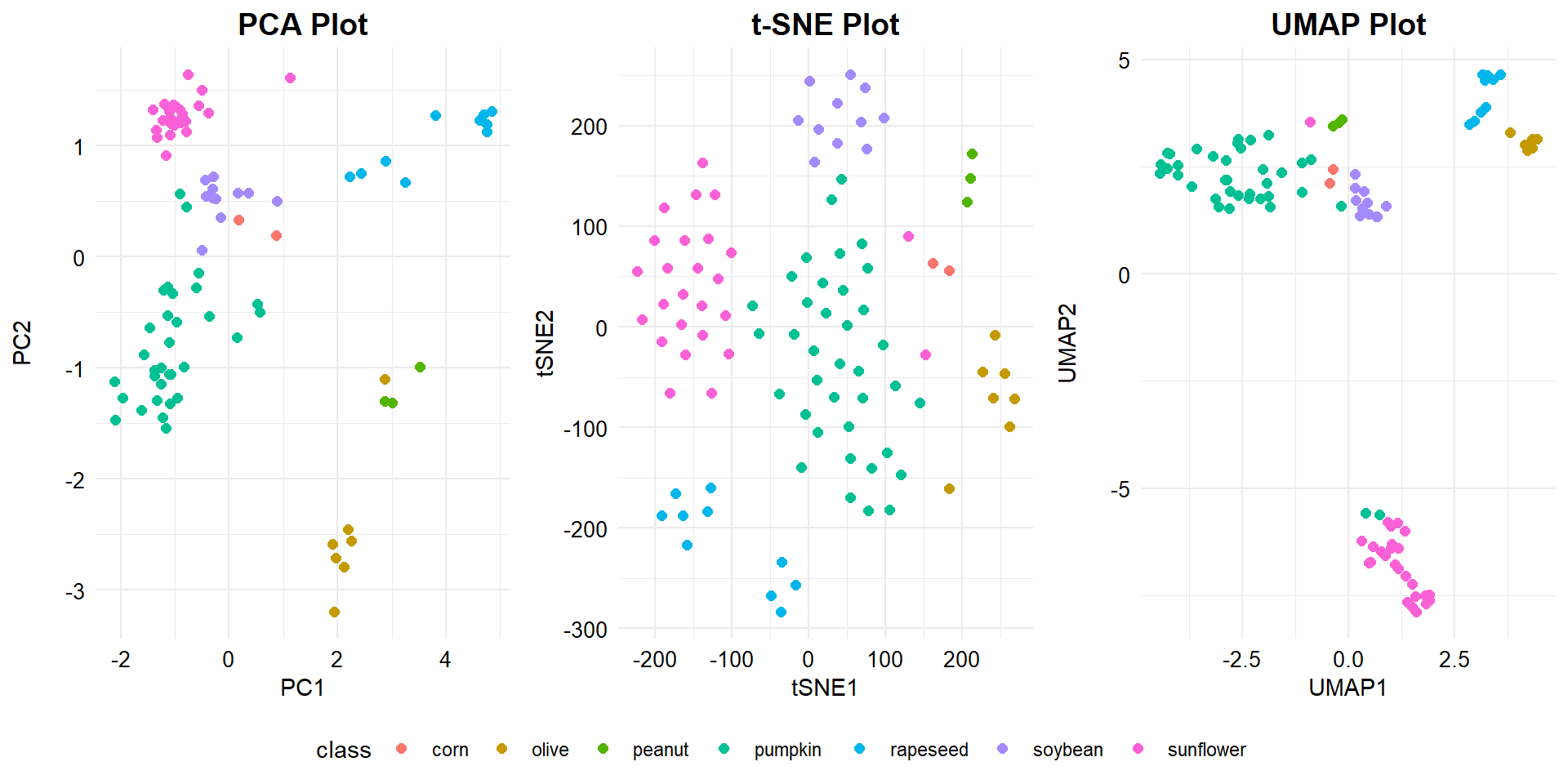
As shown in the the three plots, linear and nonlinear dimensionality reduction algorithms separate the data in the reduced space differently. Both t-SNE and UMAP offer slightly improved separation of the individual clusters beyond that provided by PCA. The separation of the sunflower oil is more pronounced using UMAP than PCA or t-SNE.

Conclusions

The t-SNE and UMAP models separate the data in the space somewhat differently to PCA. PCA is a linear dimensionality reduction algorithm whereas t-SNE and UMAP are both nonlinear algorithms. PCA assumes that the only relevant components to explain the variability in the data are the uncorrelated ones. This generally works well for multivariate Gaussian distributions. PCs have a clear and interpretable structure and therefore PCA is a widely-used method to visualize and reduce high-dimensional data. tSNE and UMAP employ local relationships between points to create a low-dimensional mapping, by comparing the full high-dimensional distance to the one in the projection subspace and capturing nonlinear structures. However, most nonlinear dimension reduction techniques (including t-SNE and UMAP) lack the strong interpretability of PCA where the dimensions are the directions of greatest variance in the source data. UMAP is similar to t-SNE but has a higher processing speed and preserves more of the global structure of the data.

There are four important hyperparameters that can impact the representations of the data that are obtained by using t-SNE and UMAP. These were not explored as part of this analysis. An automatic tuning process to choose the best combinations of the hyperparameters can be accomplished through either a grid search or random search. Alternatively, default hyperparameter values can be changed if the resulting representation doesn’t look sensible.

References

Brodnjak-Voncina, D., Kodba, Z.C., and Novic, M. 2005. Multivariate data analysis in classification of vegetable oils characterized by the content of fatty acids. Chemometrics and Intelligent Laboratory Systems 75, 31-45.

Jolliffe, I.T. 1986. Principal Component Analysis. Springer-Verlag, New York.

McInnes, L., Healy, J., and Melville, J. 2018. UMAP: Uniform manifold approximation and projection for dimension reduction. arXiv preprint arXiv:1802.03426.

Van der Maaten, L. and Hinton, G., 2008. Visualizing data using t-SNE. Journal of Machine Learning Research 9, 2579-2605.