Introduction

Estimating upper-tail threshold values, such as the 95th or 99th percentile, is critical in environmental studies because these estimates inform risk assessment and compliance decisions. Reliable estimation requires sufficiently large samples because small samples tend to produce high-variance, unstable estimates of extreme values and can miss rare events altogether. As a result, upper-tail quantiles are especially sensitive to small changes in the observed data and often require much larger sample sizes than the median to achieve comparable precision. With limited data, confidence intervals for upper-tail quantiles are wide, the estimates are less representative of the true tail behavior, and the resulting uncertainty can obscure genuine environmental risk. Larger samples reduce this uncertainty by narrowing confidence intervals, improving power to detect real changes, and lowering the chance of underestimating potentially harmful extreme contamination levels. In small-sample settings, this problem becomes more subtle: an apparently stable estimate may conceal substantial structured variability that is easy to overlook.

This post illustrates how uncertainty in estimating upper-tail quantiles varies as a function of sample size using simulation. All calculations are performed in R version 4.6.0 using several packages, including quantreg, dplyr, tidyr, and ggplot2.

Background

To understand how sample size affects the estimate of the 95th percentile (\(\tau = 0.95\)), the following simulation is conducted:

1. simulate background measurements from a right-skewed (lognormal) distribution
2. estimate a upper quantile with quantile regression
3. estimate the same upper quantile with the empirical sample quantile
4. measure the difference between the two estimators explicitly
5. use bootstrap resampling to quantify uncertainty
6. repeat the process across sample sizes

For each sample size, the simulation is repeated many times and the median estimate and its variability are summarized. The goal is not to compare methods in the large-sample limit, where both calculation methods agree, but to understand what happens when the sample size is small and the quantile of interest lies in the extreme tail.

The 95th percentile (\(\tau = 0.95\)) will be estimated using the empirical sample quantile and quantile regression. An intercept-only quantile regression model estimates specific percentiles (quantiles) of a dependent variable y without using any predictor variables, defined by

$$ y_i = \beta_0(\tau) + \epsilon_i $$

It finds the constant, \(\beta_0(\tau)\), that minimizes the check-loss function for a given quantile \(\tau\):

$$ \hat{\beta}(\tau) = min \sum_{i=1}^{n} \rho_\tau(y_i - \beta) $$

where \(\rho_\tau\) is the asymmetric check-loss function that weights residuals differently above and below zero. The solution is the value \(\hat{\beta}\) such that approximately a fraction \(\tau\) of the observations fall below it.

In this setting, quantile regression is just another way of computing the sample \(\tau\)-th quantile. In large samples, you would expect it to agree almost exactly with the empirical quantile. That expectation is correct in theory, but finite samples introduce complications.

Simulation

The simulation will investigate how well the two methods estimate the upper-tail quantile of a lognormal distribution across varying sample sizes, using repeated simulations and bootstrap resampling to assess variability and interval performance.

First, we load the required packages and fix the random-number generator state so that the simulation and bootstrap results can be reproduced.

# Load library
suppressPackageStartupMessages({
  library(quantreg)
  library(ggplot2)
  library(dplyr)
  library(tidyr)
})

# Set a seed
set.seed(123)

Next, we assign values to the parameters that will be used in the simulation. These parameters include:

• Target quantile being estimated (the 95th percentile).
• Mean and standad deviation of the lognormal distribution on the log scale.
• Range of sample sizes evaluated in the simulation, from 20 to 1000 in increments of 10.
• Number of independent simulated datasets generated for each sample size.
• Number of bootstrap resamples used within each simulated dataset to estimate uncertainty.
• Significance level for bootstrap intervals.
• Empirical quantile estimation method used in the quantile() function.

# Choose upper quantile to estimate
tau <- 0.95

# Set log-normal distribution parameters for simulated data
mu <- 3.5
sigma <- 0.25

# Define sample sizes to study
sample_sizes <- seq(20, 1000, by = 10)

# Choose how many repeated simulations to run at each sample size
nsim <- 80

# Choose how many bootstrap resamples to use inside each simulated dataset
nboot <- 200

# Set the bootstrap interval width (alpha = 0.10 gives a central 80% interval)
boot_alpha <- 0.10

# Choose which empirical quantile definition to compare against rq()
# (type = 7 is the default in quantile() and is widely used)
quantile_type <- 7

Because the data are simulated from a lognormal distribution, the true population quantile can be exactly computed and used as the reference value.

true_threshold <- qlnorm(tau, meanlog = mu, sdlog = sigma)

We define a function to fit an intercept-only quantile regression model, returing the estimated tau quantile.

fit_rq_intercept <- function(y, tau) {
  as.numeric(coef(rq(y ~ 1, tau = tau))[1])
}

We define a function to estimate bootstrap uncertainty intervals. This function bootstraps one dataset to estimate uncertainty for both the quantile regression estimate and the empirical sample quantile.

bootstrap_interval <- function(y, tau, quantile_type = 7, nboot = 200, alpha = 0.10) {
  # Record the sample size.
  n <- length(y)

  # Allocate vectors to store bootstrap estimates.
  boot_rq <- numeric(nboot)
  boot_emp <- numeric(nboot)

  # Re-sample the dataset with replacement many times.
  for (b in seq_len(nboot)) {
    # Draw a bootstrap sample.
    idx <- sample.int(n, size = n, replace = TRUE)
    yb <- y[idx]

    # Fit quantile regression to the bootstrap sample.
    boot_rq[b] <- fit_rq_intercept(yb, tau)

    # Compute the empirical sample quantile for the bootstrap sample.
    boot_emp[b] <- as.numeric(quantile(yb, probs = tau, type = quantile_type))
  }

  # Convert alpha into lower and upper tail probabilities.
  lo <- alpha / 2
  hi <- 1 - alpha / 2

  # Return percentile bootstrap intervals for both estimators.
  list(
    rq_lo = as.numeric(quantile(boot_rq, probs = lo, names = FALSE)),
    rq_hi = as.numeric(quantile(boot_rq, probs = hi, names = FALSE)),
    emp_lo = as.numeric(quantile(boot_emp, probs = lo, names = FALSE)),
    emp_hi = as.numeric(quantile(boot_emp, probs = hi, names = FALSE))
  )
}

We define a function to simulate one dataset and summarize it. This function simulates one dataset of size n, estimates the threshold in two ways, computes their difference, and computes bootstrap intervals for both estimators.

simulate_one_dataset <- function(n, tau, mu, sigma, quantile_type, nboot, boot_alpha) {
  # Generate background measurements from a skewed distribution.
  y <- rlnorm(n, meanlog = mu, sdlog = sigma)

  # Estimate the extreme quantile using quantile regression.
  rq_hat <- fit_rq_intercept(y, tau)

  # Estimate the extreme quantile empirically.
  emp_hat <- as.numeric(quantile(y, probs = tau, type = quantile_type))

  # Compute the direct difference between the two estimators.
  diff_hat <- rq_hat - emp_hat

  # Compute bootstrap bands for the current dataset.
  ci <- bootstrap_interval(y, tau, quantile_type = quantile_type, nboot = nboot, alpha = boot_alpha)

  # Store all results in one row.
  data.frame(
    n = n,
    rq_hat = rq_hat,
    emp_hat = emp_hat,
    diff_hat = diff_hat,
    rq_lo = ci$rq_lo,
    rq_hi = ci$rq_hi,
    emp_lo = ci$emp_lo,
    emp_hi = ci$emp_hi
  )
}

Now, let’s run the repeated simulations across all sample sizes. For each sample size, the simulated experiment is repeated nsim times. The results from every repetition are stacked into one dataframe.

all_results <- do.call(
  rbind,
  lapply(sample_sizes, function(n) {
    do.call(
      rbind,
      lapply(seq_len(nsim), function(s) {
        simulate_one_dataset(n, tau, mu, sigma, quantile_type, nboot, boot_alpha)
      })
    )
  })
)

Below the repeated simulations are summarized by sample size.

# Compute summary statistics
summary_by_n <- all_results %>%
  group_by(n) %>%
  summarise(
    rq_median = median(rq_hat),
    rq_q10 = quantile(rq_hat, 0.10),
    rq_q90 = quantile(rq_hat, 0.90),
    emp_median = median(emp_hat),
    emp_q10 = quantile(emp_hat, 0.10),
    emp_q90 = quantile(emp_hat, 0.90),
    diff_median = median(diff_hat),
    diff_q10 = quantile(diff_hat, 0.10),
    diff_q90 = quantile(diff_hat, 0.90),
    rq_boot_lo = median(rq_lo),
    rq_boot_hi = median(rq_hi),
    emp_boot_lo = median(emp_lo),
    emp_boot_hi = median(emp_hi),
    .groups = "drop"
  )

The figure below summarizes the simulation results, showing how the estimated 95th percentile and its associated uncertainty change as a function of sample size for both the quantile regression and empirical quantile approaches. The horizontal black line represents the true population value, while the blue line and shaded ribbon represent the quantile regression estimate and its uncertainty band, and the red line and shaded ribbon represent the empirical quantile estimate and its corresponding uncertainty band.

ggplot(summary_by_n, aes(x = n)) +
  geom_ribbon(aes(ymin = rq_boot_lo, ymax = rq_boot_hi, fill = "Quantile regression"), alpha = 0.28) +
  geom_ribbon(aes(ymin = emp_boot_lo, ymax = emp_boot_hi, fill = "Empirical quantile"), alpha = 0.28) +
  geom_line(aes(y = rq_median, color = "Quantile regression"), linewidth = 1) +
  geom_line(aes(y = emp_median, color = "Empirical quantile"), linewidth = 1) +
  geom_hline(yintercept = true_threshold, linetype = "solid", linewidth = 0.6) +
  annotate(
    "text",
    x = max(sample_sizes) - 350,
    y = true_threshold + 0.3,
    label = "True population value",
    hjust = 0,
    vjust = 0,
    size = 4.4
  ) +
  annotate(
    "text",
    x = min(sample_sizes) + 150,
    y = max(summary_by_n$rq_median) + 0.2,
    label = "Quantile regression",
    color = "blue4",
    size = 4.4
  ) +
  annotate(
    "text",
    x = 200,
    y = median(summary_by_n$emp_median) - 1,
    label = "Empirical quantile",
    color = "orangered2",
    size = 4.4
  ) +
  scale_color_manual(
    values = c(
      "Quantile regression" = "blue4",
      "Empirical quantile" = "orangered2"
    )
  ) +
  scale_fill_manual(
    values = c(
      "Quantile regression" = "blue4",
      "Empirical quantile" = "orangered2"
    )
  ) +
  labs(
    title = "Quantile estimations of small random samples",
    x = "sample size",
    y = paste0("estimated ", tau, " quantile")
  ) +
  theme_classic(base_size = 12) +
  theme(
    plot.title = element_text(face = "bold", hjust = 0.5),
    legend.title = element_blank(),
    legend.position = "none",
    axis.title.y = element_text(angle = 90)
  )

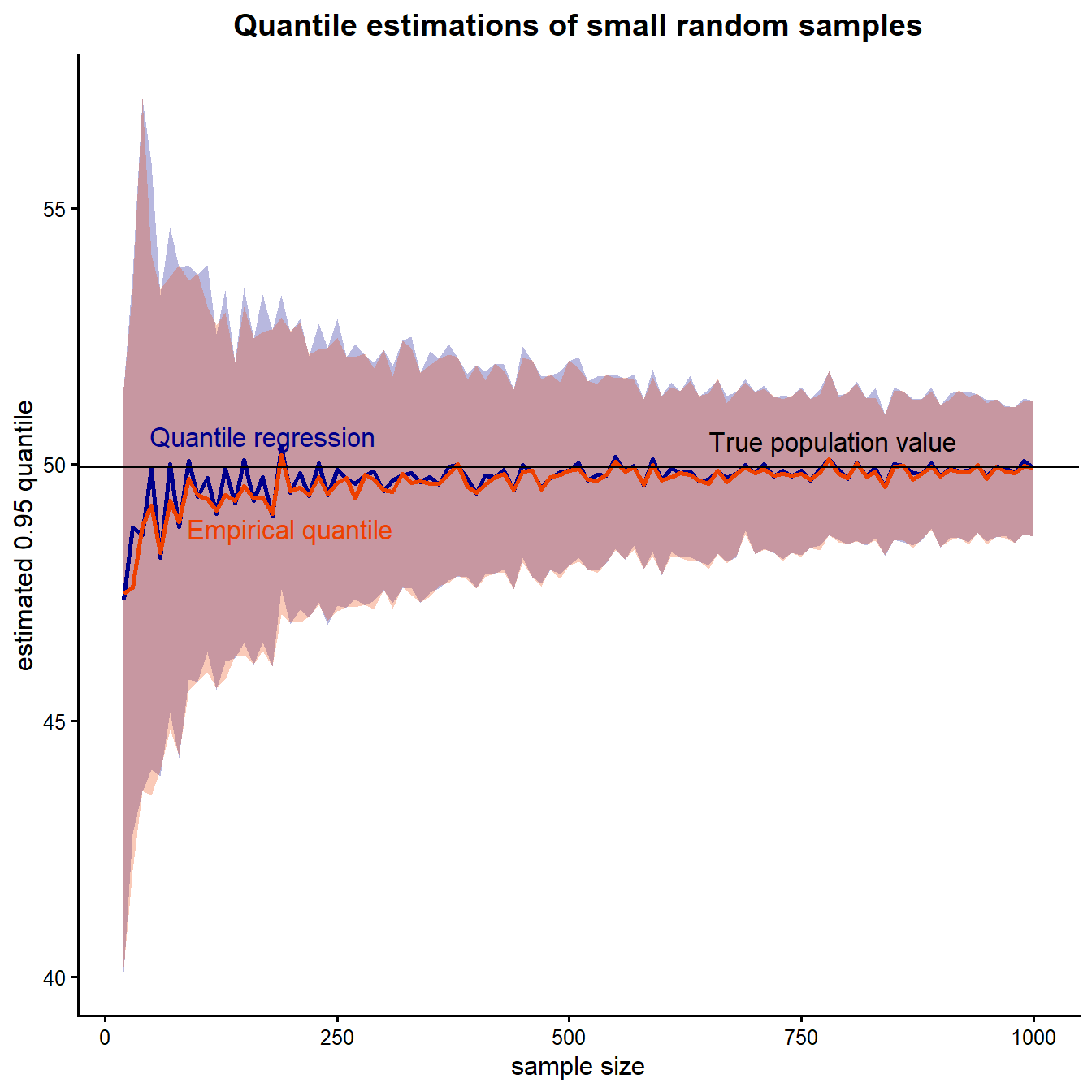
Estimating threshold values from small datasets is inherently uncertain, especially when the quantity of interest lies near the extreme end of the distribution. Although both methods converge toward the true value as sample size increases, the figure highlights an important practical point: when sample sizes are small, upper-tail estimates can vary substantially from one dataset to another. This variability reflects the limited information available in the extreme tail of the distribution, where the estimate is often determined by only a few of the largest observations.

The figure also demonstrates that even methods that are theoretically similar can exhibit subtle finite-sample differences. Quantile regression and empirical quantiles target the same underlying population percentile, yet their uncertainty patterns differ slightly because of how each method treats order statistics and interpolation in small samples. Together, these results emphasize why uncertainty should be considered explicitly when using upper-tail statistics to establish background thresholds or screening criteria.

In the figure below, the quantile regression estimate is compared with the empirical quantile estimate directly by plotting their difference as a function of sample size. Positive values mean the quantile regression estimate is larger; negative values mean the empirical quantile estimate is larger. Although both methods estimate the same theoretical 95th percentile, the figure reveals a structured oscillating pattern in their finite-sample behavior. The black line represents the median difference across repeated simulations, while the shaded gray region shows the central range of variability.

ggplot(summary_by_n, aes(x = n)) +
  geom_ribbon(aes(ymin = diff_q10, ymax = diff_q90), alpha = 0.2, fill = "gray70") +
  geom_line(aes(y = diff_median), linewidth = 1) +
  geom_hline(yintercept = 0, linetype = "dashed", linewidth = 0.6) +
  labs(
    title = paste0("Difference between rq() and quantile(type = ", quantile_type, ")"),
    x = "sample size",
    y = "rq() - quantile()"
  ) +
  theme_classic(base_size = 12) +
  theme(
    plot.title = element_text(face = "bold", hjust = 0.5)
  )

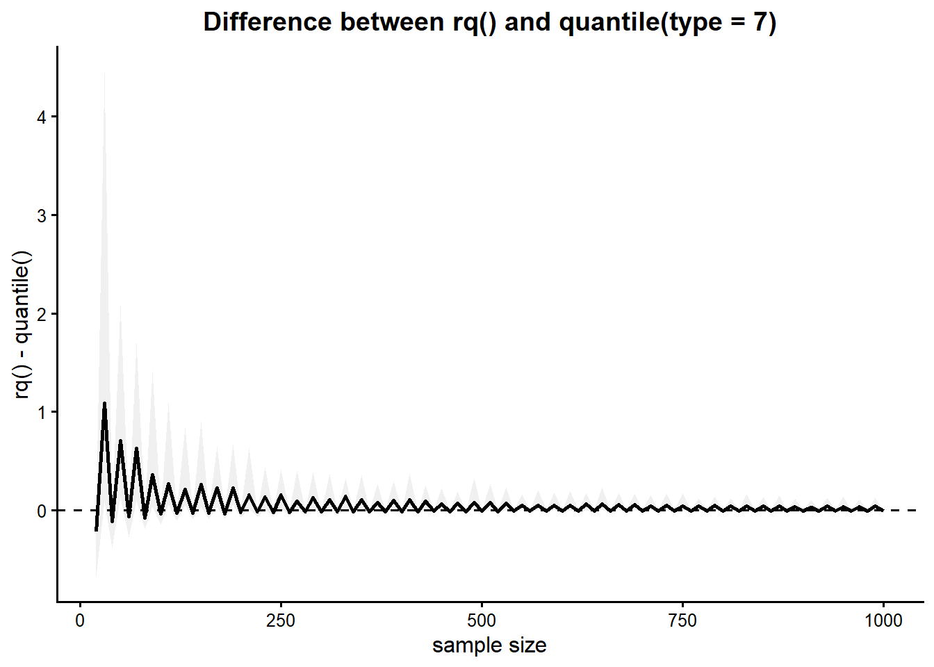
The difference between the quantile regression estimate and the empirical quantile estimate is not random, but follows a systematic oscillating pattern at small sample sizes. Although both methods target the same theoretical 95th percentile, their finite-sample implementations behave differently because the empirical quantile relies on interpolation between adjacent order statistics, whereas the quantile regression estimate is obtained through optimization of the quantile loss function.

The oscillation is largest at small sample sizes, where the upper-tail estimate is controlled by only a few extreme observations. In this regime, small changes in interpolation can produce noticeable shifts in the estimated threshold. As sample size increases, the oscillation gradually decreases in magnitude and the difference between the two methods approaches zero. This occurs because the upper order statistics become more densely spaced, reducing the influence of interpolation and stabilizing both estimators.

The oscillating behavior observed in the difference between the quantile regression and empirical quantile estimates can be explained by examining the fractional component of the empirical quantile index. Empirical quantiles are computed using an index:

$$ k = \tau(n - 1) + 1 $$

For \(\tau = 0.95\), this determines where the 95th percentile falls within the ordered data. If k is an integer, the quantile corresponds exactly to one of the observed values. If not, the estimate is obtained by interpolating between two adjacent observations. The amount of interpolation depends on the fractional part of k. Because sample sizes increase in steps of 10 and \(\tau = 0.95\) or 19/20, the fractional component alternates predictably between approximately 0.05 and 0.55. This deterministic pattern controls the degree of interpolation used in the empirical quantile calculation and provides the underlying explanation for the repeating oscillation observed in the previous figure.

The figure illustrates two important points. First, finite-sample differences between theoretically equivalent quantile estimators can produce structured, predictable behavior rather than simple random variation. Second, and more importantly, it highlights the large uncertainty associated with estimating upper-tail thresholds from small datasets. Even when the average estimate appears stable, the variability around that estimate can remain substantial at low sample sizes, emphasizing the need for caution when using upper-tail threshold values to define background.

The next plot shows the fractional part of the target quantile index used by the empirical quantile definition as a function of sample size.

# Get fractional component
summary_by_n <- summary_by_n %>%
  mutate(
    quantile_index = tau * (n - 1) + 1,
    fractional_index = quantile_index %% 1
  )

# Create plot
ggplot(summary_by_n, aes(x = n, y = fractional_index)) +
  geom_line(linewidth = 1) +
  geom_point(size = 1.6) +
  geom_hline(yintercept = 0, linetype = "dashed", linewidth = 0.6) +
  labs(
    title = paste0("Fractional index for tau = ", tau),
    x = "sample size",
    y = "fractional part of tau * (n - 1) + 1"
  ) +
  theme_classic(base_size = 12) +
  theme(
    plot.title = element_text(face = "bold", hjust = 0.5)
  )

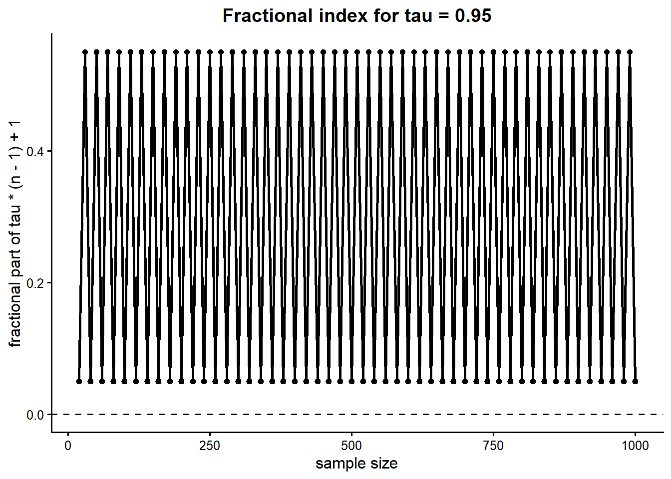
The fractional component of the empirical quantile index does not vary randomly with sample size, but instead follows a highly structured and deterministic pattern. When the fractional component is close to zero, the empirical quantile lies near an actual order statistic, requiring little interpolation. When the fractional component is closer to 0.5, the estimate falls midway between two order statistics and interpolation plays a larger role.

While the oscillation itself is mathematically interesting, the more important point is what it reveals about uncertainty. At small sample sizes, the 95th percentile is effectively determined by one or two of the largest observations. Small changes in how those observations are weighted or interpolated can produce noticeable differences in the estimated threshold. As the sample size increases, the largest observations become more densely spaced, and the effect of interpolation diminishes. This is why both the oscillation and the overall uncertainty shrink with increasing n. However, in the small-sample regime, the regime that often matters most in practice, the uncertainty is large, and the estimates are sensitive to methodological details.

While the interpolation-driven oscillation helps explain the structured finite-sample behavior observed in the simulation, in many environmental applications, uncertainty arising from distributional misspecification, censoring and nondetect handling, spatial heterogeneity, temporal dependence, outliers, and sampling bias is often substantially larger than the interpolation effects illustrated here. The primary purpose of this example is therefore not to suggest that interpolation dominates real-world uncertainty, but rather to illustrate how small-sample upper-tail estimation can exhibit structured sensitivity to methodological details.

Final Thoughts

This simulation highlights that even when two methods are theoretically equivalent, their finite-sample behavior can differ in structured and meaningful ways. For upper-tail quantiles, such as the 95th percentile, these differences are amplified by the scarcity of data in the tail. The result is not just random variability, but a combination of wide uncertainty due to limited data and systematic effects tied to how quantiles are defined. The interpolation effects illustrated here are mainly useful as an example of how small-sample upper-tail estimates can exhibit structured methodological sensitivity. In practice, other sources of uncertainty, including distributional assumptions, nondetect handling, spatial variability, temporal dependence, outliers, and sampling bias, are often more important.

When using upper-tail quantiles to define thresholds, it is important to recognize that the estimate itself is only part of the story. The uncertainty around that estimate, and the sensitivity to methodological choices, can be just as important. In practice, this means that sparse datasets should be treated with caution when estimating upper-tail threshold values. The apparent precision of a single number can be misleading, especially when that number is determined by only a few extreme observations. Understanding these limitations helps ensure that threshold decisions are grounded not just in point estimates, but in a realistic view of their uncertainty.

This is particularly important because many background threshold values are calculated as a 95 percent upper confidence limit on the 95th percentile (95-95 UTL) of the assumed background parent population. A 95-95 UTL is even more demanding than estimating a pointwise 95th percentile because it adds a confidence requirement on top of the percentile coverage requirement. As a result, the sample size needed for a reliable 95-95 UTL is typically much larger than the sample size needed for a stable point estimate of the 95th percentile.