Natural Neighbor Interpolation With R
By Charles Holbert
May 22, 2023
Introduction
Kriging is an exact interpolator which uses geostatistical techniques to calculate the autocorrelation between data points, and produce a minimum variance unbiased estimate, taking in consideration the spatial configuration of the underlying phenomenon. Before performing the kriging, a variographic study has to be done. Based on the experimental variogram (obtained from the input data set), an appropriate variogram model and adequate parameters have to be chosen. The variogram model mathematically specifies the spatial variability of the data set and the resulting grid file. The interpolation weights, which are applied to data points during the grid node calculations, are direct functions of the variogram model. When the variogram is specified for kriging, the following parameters have to be set: sill, range, and nugget, but also the anisotropy information. The development of an appropriate variogram model for a data set requires the understanding and application of advanced statistical concepts. This can be challenging, especially for inexperienced users.
An alternative spatial interpolation method is natural neighbor interpolation. Natural neighbor interpolation finds the closest subset of input samples to a query point and applies weights to them based on proportionate areas in order to interpolate a value (Sibson 1981). It adapts locally to the structure of the input data, requiring no input from the user pertaining to search radius, sample count, or shape. This post presents and demonstrates several methods for natural neighbor interpolation using the R language for statistical computing and visualization. The results will be compared to those obtain using ordinary kriging.
Preliminaries
We’ll start by loading the required R libraries.
# Load libraries
library(dplyr)
library(ggplot2)
library(scales)
library(sp)
library(gstat)
library(raster)
Let’s set the European Petroleum Survey Group (EPSG) code for our data. The EPSG code is a unique identifier for different coordinate systems. It’s a public registry of geodetic datums, spatial reference systems, Earth ellipsoids, coordinate transformations, and related units of measurement. Each entity is assigned an EPSG code between 1024-32767.
# Set EPSG code
epsg <- 28992
Let’s create a few functions that can be used to create either a rectilinear grid or a grid based on the convex hull of the data.
# Function to expand poly
expandpoly <- function(mypol, fact) {
  m1 <- mean(mypol[, 1])
  m2 <- mean(mypol[, 2])
  cbind((mypol[, 1] - m1) * fact + m1, (mypol[, 2] - m2) * fact + m2)
}

# Function to create 2D grid
get_grid <- function(d, nodes = 200, grid_method = 'rect',
  expand = 'Y', fx = 0.1, fy = 0.1, epsg) {

  d <- data.frame(d)

  # Make data geospatial object
  coordinates(d) = ~x+y
  proj4string(d) = CRS(paste0("+init=epsg:", epsg))
  n <- length(d@coords[,1])	# no. of data points

  # Setup grid automatically using data extents
  delx <- (max(d@coords[,1]) - min(d@coords[,1])) * fx
  dely <- (max(d@coords[,2]) - min(d@coords[,2])) * fy

  if (expand == 'Y') {
    xb <- round(min(d@coords[,1]) - delx, -1)
    xe <- round(max(d@coords[,1]) + delx, -1)
    yb <- round(min(d@coords[,2]) - dely, -1)
    ye <- round(max(d@coords[,2]) + dely, -1)
  } else {
    xb <- min(d@coords[,1])
    xe <- max(d@coords[,1])
    yb <- min(d@coords[,2])
    ye <- max(d@coords[,2])
  }

  xn <- (xe - xb)/nodes
  yn <- (ye - yb)/nodes

  # Create rectangular grid and make spatial object
  if (grid_method == 'rect') {
    grid2D <- expand.grid(x = seq(xb, xe, xn), y = seq(yb, ye, yn))
    gridded(grid2D) <- ~x+y
    proj4string(grid2D) = CRS(paste0("+init=epsg:", epsg))
  }

  # Create grid based on hull points and make spatial object
  if (grid_method == 'hull') {
    ma <- as.matrix(d@coords)
    ma <- ma[chull(d@coords),, drop = F]
    ma.expand <- ma
    if (expand == 'Y') ma.expand <- expandpoly(ma, fact = 1 + fx)
    grid2D <- splancs::gridpts(ma.expand, xs = xn, ys = yn)
    grid2D <- data.frame(grid2D)
    colnames(grid2D) <- c("x", "y")
    gridded(grid2D) <- ~x+y
    proj4string(grid2D) = CRS(paste0("+init=epsg:", epsg))
  }

  return(list(grid = grid2D, xn = xn, yn = yn))
}
Data
This post uses the meuse data set included in the R gstat library. The data are comprised of locations and top soil heavy metal concentrations (parts-per-million [ppm]), along with a number of soil and landscape variables, collected in a flood plain of the river Meuse, near the village Stein in the Netherlands. Heavy metal concentrations are bulk sampled from an area of approximately 15 meters by 15 meters. Coordinates are in Rijksdriehoek (RDH) (Netherlands topographical) map coordinates.
# Load data
data(meuse)

# Inspect structure of the data
str(meuse)
## 'data.frame':	155 obs. of  14 variables:
##  $ x      : num  181072 181025 181165 181298 181307 ...
##  $ y      : num  333611 333558 333537 333484 333330 ...
##  $ cadmium: num  11.7 8.6 6.5 2.6 2.8 3 3.2 2.8 2.4 1.6 ...
##  $ copper : num  85 81 68 81 48 61 31 29 37 24 ...
##  $ lead   : num  299 277 199 116 117 137 132 150 133 80 ...
##  $ zinc   : num  1022 1141 640 257 269 ...
##  $ elev   : num  7.91 6.98 7.8 7.66 7.48 ...
##  $ dist   : num  0.00136 0.01222 0.10303 0.19009 0.27709 ...
##  $ om     : num  13.6 14 13 8 8.7 7.8 9.2 9.5 10.6 6.3 ...
##  $ ffreq  : Factor w/ 3 levels "1","2","3": 1 1 1 1 1 1 1 1 1 1 ...
##  $ soil   : Factor w/ 3 levels "1","2","3": 1 1 1 2 2 2 2 1 1 2 ...
##  $ lime   : Factor w/ 2 levels "0","1": 2 2 2 1 1 1 1 1 1 1 ...
##  $ landuse: Factor w/ 15 levels "Aa","Ab","Ag",..: 4 4 4 11 4 11 4 2 2 15 ...
##  $ dist.m : num  50 30 150 270 380 470 240 120 240 420 ...
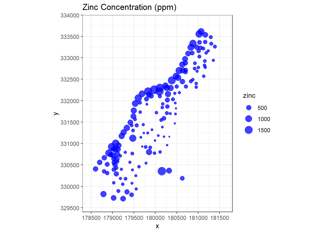
Let’s visually inspect how zinc concentrations vary over the domain of interest where concentration is related to point size.
# Visually inspect how zinc varies over domain of interest
meuse %>%
  as.data.frame %>%
  ggplot(aes(x, y)) +
  geom_point(aes(size = zinc), color = 'blue', alpha = 3/4) +
  ggtitle('Zinc Concentration (ppm)') +
  scale_x_continuous(limits = c(178300, 181800),
                     breaks = seq(178500, 181500, by = 500),
                     expand = c(0, 0)) +
  scale_y_continuous(limits = c(329400, 334000),
                     breaks = seq(329500, 334000, by = 500),
                     expand = c(0, 0)) +
  coord_equal() +
  theme_bw()
Let’s convert the meuse data frame to a SpatialPointsDataFrame. The difference between SpatialPoints and SpatialPointsDataFrame are the attributes that are associated with the points. SpatialPointsDataFrames have additional information associated with the points while SpatialPoints contain only the spatial information about the point. We will assign the projection system using the EPSG code.
# Convert data to a spatial points dataframe
meuse.spdf <- meuse
coordinates(meuse.spdf) <- ~ x + y
proj4string(meuse.spdf) = CRS(paste0("+init=epsg:", epsg))
We can use the slot command to retreive the projection attributes.
slot(meuse.spdf, 'proj4string')
## Coordinate Reference System:
## Deprecated Proj.4 representation:
##  +proj=sterea +lat_0=52.1561605555556 +lon_0=5.38763888888889
## +k=0.9999079 +x_0=155000 +y_0=463000 +ellps=bessel +units=m +no_defs
## WKT2 2019 representation:
## PROJCRS["Amersfoort / RD New",
##     BASEGEOGCRS["Amersfoort",
##         DATUM["Amersfoort",
##             ELLIPSOID["Bessel 1841",6377397.155,299.1528128,
##                 LENGTHUNIT["metre",1]]],
##         PRIMEM["Greenwich",0,
##             ANGLEUNIT["degree",0.0174532925199433]],
##         ID["EPSG",4289]],
##     CONVERSION["RD New",
##         METHOD["Oblique Stereographic",
##             ID["EPSG",9809]],
##         PARAMETER["Latitude of natural origin",52.1561605555556,
##             ANGLEUNIT["degree",0.0174532925199433],
##             ID["EPSG",8801]],
##         PARAMETER["Longitude of natural origin",5.38763888888889,
##             ANGLEUNIT["degree",0.0174532925199433],
##             ID["EPSG",8802]],
##         PARAMETER["Scale factor at natural origin",0.9999079,
##             SCALEUNIT["unity",1],
##             ID["EPSG",8805]],
##         PARAMETER["False easting",155000,
##             LENGTHUNIT["metre",1],
##             ID["EPSG",8806]],
##         PARAMETER["False northing",463000,
##             LENGTHUNIT["metre",1],
##             ID["EPSG",8807]],
##         ID["EPSG",19914]],
##     CS[Cartesian,2],
##         AXIS["(E)",east,
##             ORDER[1],
##             LENGTHUNIT["metre",1,
##                 ID["EPSG",9001]]],
##         AXIS["(N)",north,
##             ORDER[2],
##             LENGTHUNIT["metre",1,
##                 ID["EPSG",9001]]],
##     USAGE[
##         SCOPE["unknown"],
##         AREA["Netherlands - onshore, including Waddenzee, Dutch Wadden Islands and 12-mile offshore coastal zone."],
##         BBOX[50.75,3.2,53.7,7.22]]]
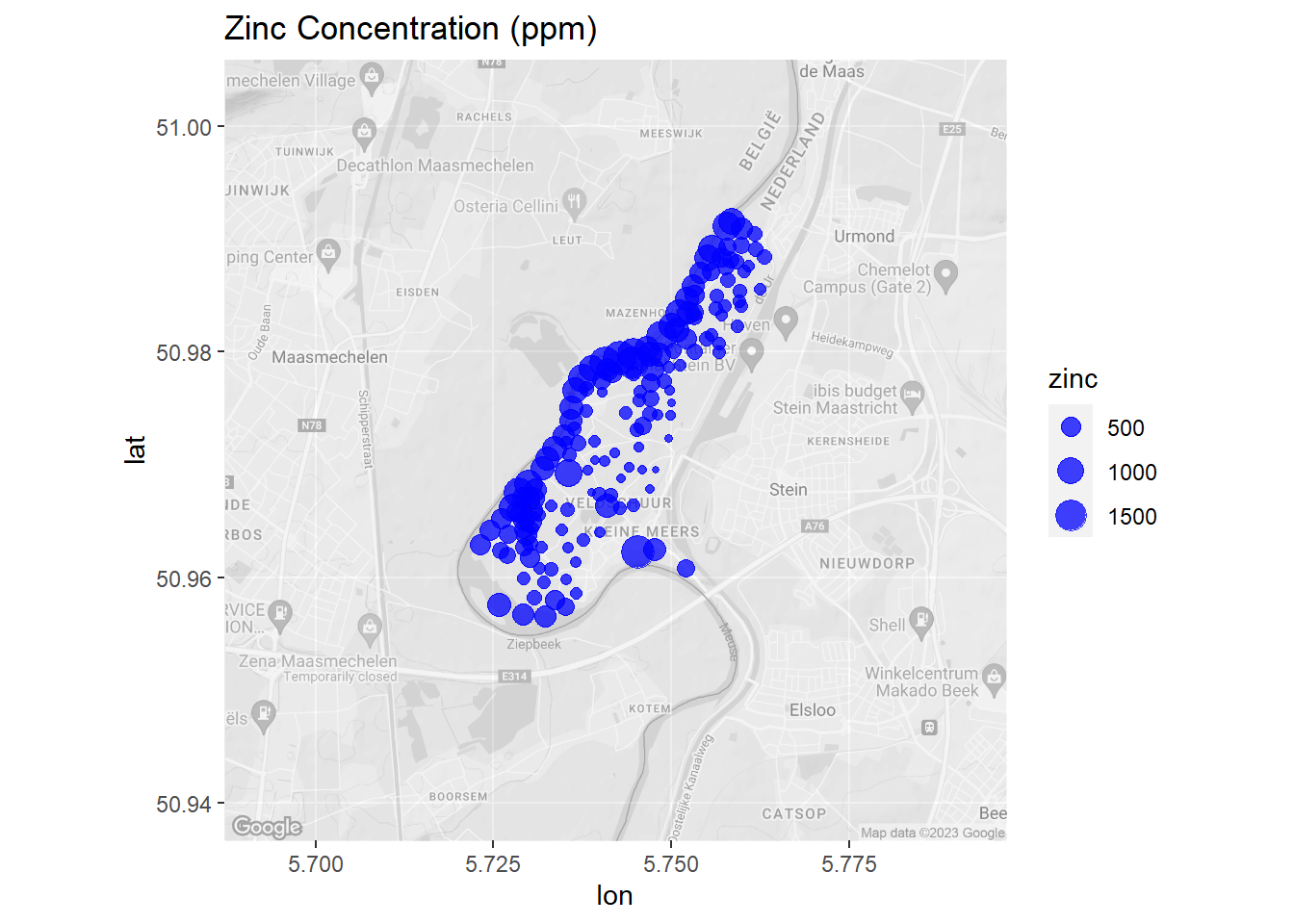
Now, let’s create a map of zinc concentrations that includes a basemap showing the local terrain.
# Load library
library(ggmap)

# Get Google map
meuse_basemap <- get_map(
  location = c(lon = 5.742061, lat = 50.971337),
  source = 'google', maptype = 'terrain', color = 'bw',
  crop = FALSE, zoom = 13
)

# Modify the ggmap to make it transparent. Save the attributes as an object so
# that they can be reassigned.
meuse_basemap_attributes <- attributes(meuse_basemap)

# Create matrix same dimensions as Google basemap, but with the color hex codes
# in each cell adjusted to half transparency.
meuse_basemap_transparent <- matrix(
  adjustcolor(meuse_basemap, alpha.f = 0.5),
  nrow = nrow(meuse_basemap)
)

# Assign attributes to modified matrix to turn it back into a usable ggmap
attributes(meuse_basemap_transparent) <- meuse_basemap_attributes

# Convert meuse to lat long
WGS84 <- CRS("+init=epsg:4326")
meuse.latlon <- spTransform(meuse.spdf, WGS84) %>%
  data.frame()

# Create map
ggmap(meuse_basemap_transparent) +
  geom_point(data = meuse.latlon, aes(x = x, y = y, size = zinc),
  color = 'blue', alpha = 3/4) +
  ggtitle('Zinc Concentration (ppm)')
Kriging
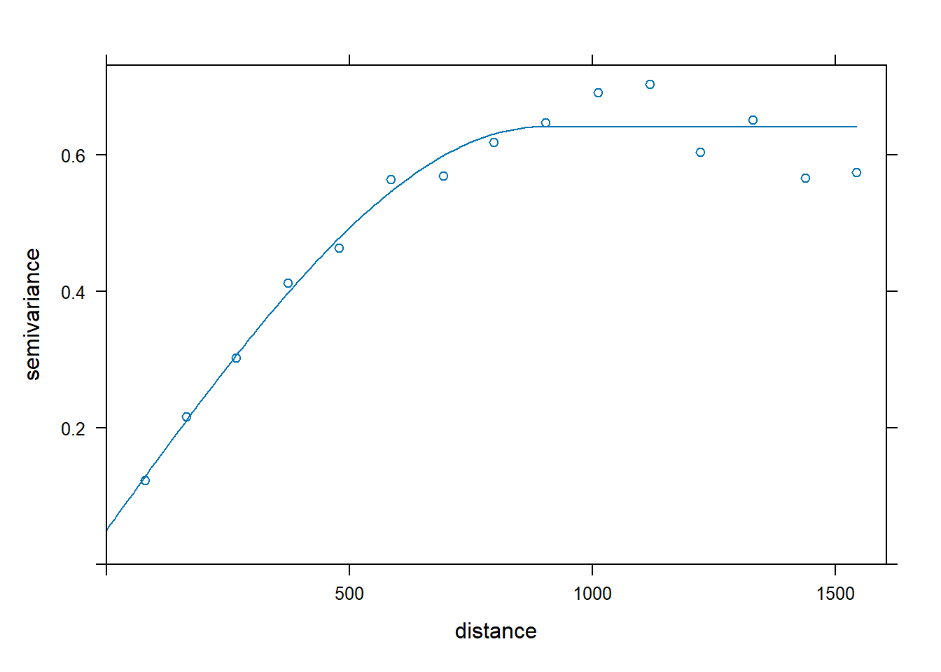
Let’s use ordinary kriging (Isaaks and Srivastava 1989; Gooevaerts 1997) to model zinc concentrations across the investigative area. Kriging is an interpolation technique that calculates a concentration at an unknown location through a weighted average of known points within a data-specific neighborhood. The interpolation weights, which are applied to data points during the grid node calculations, are direct functions of the variogram model. Let’s define and plot the variogram model.
# Fit variogram
lzn.vgm <- variogram(log(zinc) ~ 1, meuse.spdf)
lzn.fit <- fit.variogram(lzn.vgm, model = vgm(1, 'Sph', 900, 1))

# Plot variogram
plot(lzn.vgm, lzn.fit)
Let’s create a grid for interpolation based on the convex hull of the data.
# Create grid
grid2D <- get_grid(
  d = meuse,
  nodes = 200,
  grid_method = 'hull',
  expand = 'N',
  fx = 0.1, fy = 0.1,
  epsg = epsg
)
str(grid2D)
## List of 3
##  $ grid:Formal class 'SpatialPixels' [package "sp"] with 5 slots
##   .. ..@ grid       :Formal class 'GridTopology' [package "sp"] with 3 slots
##   .. .. .. ..@ cellcentre.offset: Named num [1:2] 178612 329724
##   .. .. .. .. ..- attr(*, "names")= chr [1:2] "x" "y"
##   .. .. .. ..@ cellsize         : Named num [1:2] 13.9 19.5
##   .. .. .. .. ..- attr(*, "names")= chr [1:2] "x" "y"
##   .. .. .. ..@ cells.dim        : Named int [1:2] 200 200
##   .. .. .. .. ..- attr(*, "names")= chr [1:2] "x" "y"
##   .. ..@ grid.index : int [1:19992] 39839 39840 39841 39842 39843 39844 39845 39846 39847 39848 ...
##   .. ..@ coords     : num [1:19992, 1:2] 179141 179155 179169 179183 179197 ...
##   .. .. ..- attr(*, "dimnames")=List of 2
##   .. .. .. ..$ : chr [1:19992] "1" "2" "3" "4" ...
##   .. .. .. ..$ : chr [1:2] "x" "y"
##   .. ..@ bbox       : num [1:2, 1:2] 178605 329714 181390 333611
##   .. .. ..- attr(*, "dimnames")=List of 2
##   .. .. .. ..$ : chr [1:2] "x" "y"
##   .. .. .. ..$ : chr [1:2] "min" "max"
##   .. ..@ proj4string:Formal class 'CRS' [package "sp"] with 1 slot
##   .. .. .. ..@ projargs: chr "+proj=sterea +lat_0=52.1561605555556 +lon_0=5.38763888888889 +k=0.9999079 +x_0=155000 +y_0=463000 +ellps=bessel"| __truncated__
##   .. .. .. ..$ comment: chr "PROJCRS[\"Amersfoort / RD New\",\n    BASEGEOGCRS[\"Amersfoort\",\n        DATUM[\"Amersfoort\",\n            E"| __truncated__
##  $ xn  : num 13.9
##  $ yn  : num 19.5
The grid consists of 19,992 cells with a cell size of 13.9 meters in the x-direction and 19.5 meters in the y-direction.
Now, let’s use the gstat library to krige the zinc concentration data over our grid using the model variogram. The krige() function can be used for simple, ordinary or universal kriging (sometimes called external drift kriging); kriging in a local neighborhood, point kriging or kriging of block mean values (rectangular or irregularblocks); and conditional (Gaussian or indicator) simulation for all kriging varieties. It also can be used for inverse distance weighted interpolation. For ordinary and simple kriging, we use the formula z ~ 1. We’ll use natural log transformed data to stabilize the variance in the zinc concentration data.
# Perform ordinary kriging
zn.kriged <- krige(log(zinc) ~ 1, meuse.spdf, grid2D$grid, model = lzn.fit)
## [using ordinary kriging]
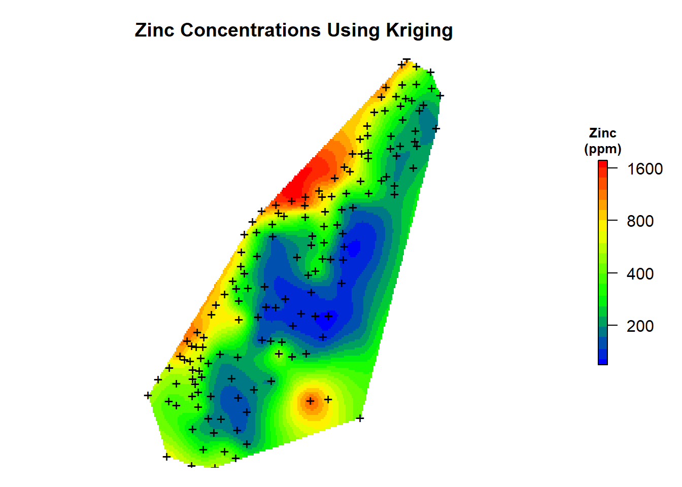
Let’s inspect a map of the kriging predictions.
# Create color-scale for plot
leg <- c(
  "#0000ff", "#0028d7", "#0050af", "#007986", "#00a15e",
  "#00ca35", "#00f20d", "#1aff00", "#43ff00", "#6bff00",
  "#94ff00", "#bcff00", "#e5ff00", "#fff200", "#ffca00",
  "#ffa100", "#ff7900", "#ff5000", "#ff2800", "#ff0000"
)

# Create breaks for legend
axis.ls <- list(
  at = log10(c(100, 200, 400, 800, 1600)),
  labels = c(100, 200, 400, 800, 1600)
)

# Convert grid from from SpatialPointsDataFrame to SpatialPixelsDataFrame
meusegrid.spdf <- SpatialPixelsDataFrame(
  grid2D$grid,
  data = data.frame(grid2D$grid)
)

# Add predictions to spatial pixels object
meusegrid.spdf$zn.krige <- exp(zn.kriged$var1.pred)

# Create plot
par(mar = c(1, 1, 3, 2))  # bottom, left, top, right; default is c(5.1, 4.1, 4.1, 2.1)
plot(
  log10(raster(meusegrid.spdf['zn.krige'])),
  col = leg,
  main = 'Zinc Concentrations Using Kriging',
  axes = FALSE,
  box = FALSE,
  axis.args = axis.ls,
  legend.args = list(text = "Zinc\n(ppm)", side = 3, font = 2, line = 0.2, cex = 0.8)
)
points(coordinates(meuse.spdf), pch = "+")
Natural Neighbor Interpolation
The natural neighbor method interpolates grid values by weighting neighboring data points based on proportionate areas. The natural neighbors of any point are those associated with neighboring Thiessen polygons, also known as Voronoi polygons. Initially, Thiessen polygons are constructed for all given points. If a new point (target) were added to the data set, these Thiessen polygons would be modified. In fact, some of the polygons would shrink in size, while none would increase in size. The area associated with the target’s Thiessen polygon that was taken from an existing polygon is called the “borrowed area.” The natural neighbor interpolation algorithm uses a weighted average of the neighboring observations, where the weights are proportional to the “borrowed area.”
The use of the term “natural” to describe the interpolation technique was introduced by its developer Robin Sibson (1981), who characterizes the technique with the following description:
All interpolation methods involve to some extent the idea that the value of the interpolant at a point should depend more on data values at nearby data sites than at distant ones. In natural-neighbor interpolation the idea of ’neighbor’ in a spatial configuration is formalized in a natural way and made quantitative, and the properties of the method depend on an apparently new geometric identity relating this quantitative measure of ’neighborliness’ to position.
The unifying concept is that natural neighbor interpolation derives from fundamental geometric principles and not through an artificial construct.
The basic equation is given by the following:
$$G(x) = \sum_{i=1}^{n}w_{i}(x)f(x_{i})$$
where G(x) is the estimate at \(x_{i}\), \(w_{i}\) are the weights, and \(f(x_{i})\) are the known data at \(x_{i}\). The weights, \(w_{i}\), are calculated by finding how much of each of the surrounding areas is “stolen” when inserting x into the tessellation:
$$w_{i}(x) = \frac{A(x_{i})}{A(x)}$$
where A(x) is the volume of the new cell centered in x, and \(A(x_{i})\) is the volume of the intersection between the new cell centered in x and the old cell centered in \(x_{i}\).
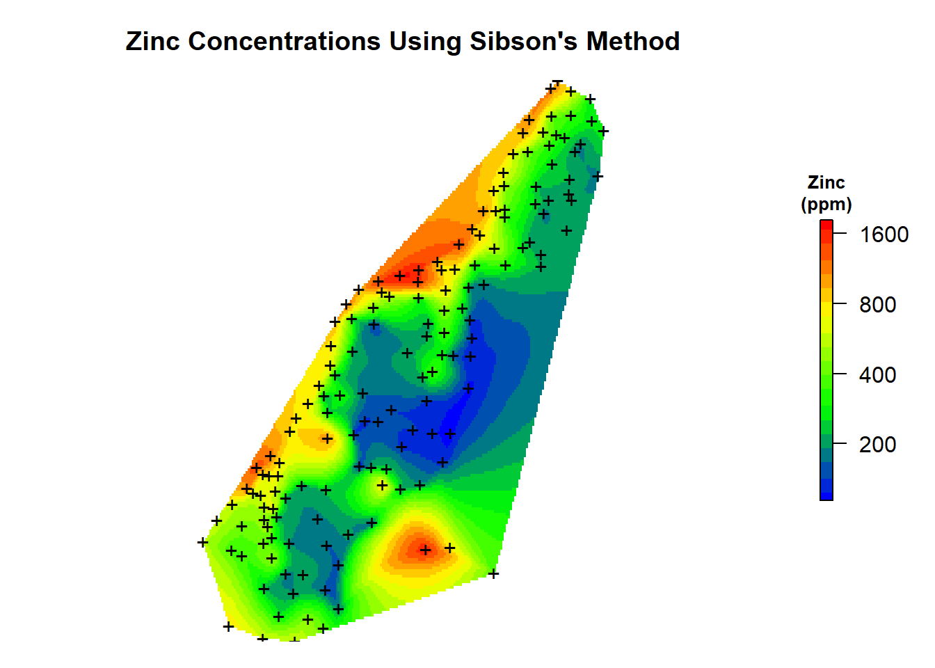
Natural Neighbor Interpolation Using Sibson’s Method
As discussed above, Sibson’s natural neighbor interpolation uses a weighted average of the neighboring observations. These natural neighbors are determined by finding which Voronoi regions from the original point set would intersect the Voronoi region of the interpolation point, if it were to be inserted. The resulting function is continuous everywhere within the convex hull of the sample set.
First, let’s create a function that generates the Voronoi polygons.
# Load libraries
library(deldir)
library(rgeos)

# Function to create Voronoi polygons
voronoipolygons <- function(x) {
  if (.hasSlot(x, 'coords')) {
    crds <- x@coords
  } else crds <- x
  z <- deldir(crds[, 1], crds[, 2])
  w <- tile.list(z)
  polys <- vector(mode = 'list', length = length(w))
  for (i in seq(along = polys)) {
    pcrds <- cbind(w[[i]]$x, w[[i]]$y)
    pcrds <- rbind(pcrds, pcrds[1, ])
    polys[[i]] <- Polygons(list(Polygon(pcrds)), ID = as.character(i))
  }
  SP <- SpatialPolygons(polys)
  voronoi <- SpatialPolygonsDataFrame(
    SP,
    data = data.frame(
      x = crds[, 1],
      y = crds[,2],
      row.names = sapply(slot(SP, 'polygons'), function(x) slot(x, 'ID'))
    )
  )
}
Second, let’s extract the coordinates of the sample locations and the zinc concentration data.
# Get locations
myvars <- c('x', 'y')
dat <- meuse[, myvars]

# Get zinc data
zn <- meuse[,6]
Now, let’s create Voronoi polygons for the sampled locations.
# Create polygons
v2 <- voronoipolygons(dat)

# Add projection to polygons
proj4string(v2) <- CRS(paste0("+init=epsg:", epsg))
Finally, let’s perform natural neighbor interpolation using Sibson’s method. A word of caution is that this algorithm is computationally intensive and with a grid size of 200 nodes by 200 nodes, this will take several hours to run.
# Initialize parameters
predgrid <- as.data.frame(grid2D$grid)
n <- nrow(dat)
N <- nrow(predgrid)
int <- matrix(nrow = N, ncol = n)
loc <- as.matrix(cbind(predgrid[,1:2]))

# Loop over prediction grid to get Sibson weights
for (i in 1:N){
  loc.temp <- rbind(dat, loc[i,])
  vor.temp <- voronoipolygons(loc.temp)
  proj4string(vor.temp) <- CRS(paste0("+init=epsg:", epsg))
  for (j in 1:n){
    s <- gIntersection(
      SpatialPolygons(vor.temp@polygons[n+1]),
      SpatialPolygons(v2@polygons[j])
    )
    if(is.null(s)) {
      int[i,j] = 0
    } else {
      new.area <- vor.temp@polygons[[n+1]]@Polygons[[1]]@area
      int[i,j] <- gArea(s) / new.area
    }
  }
}

# Get predictions
pred <- rowSums(sweep(int, MARGIN = 2, zn, '*'))
zn.sibson <- cbind(as.data.frame(loc), pred = pred)
Now, let’s add the predictions to our spatial pixels object and create a map of the natural neighbor predictions that were made using Sibson’s method.
# Add predictions to spatial pixels object
meusegrid.spdf$zn.sibson <- zn.sibson$pred

# Create plot
par(mar = c(1, 1, 3, 2))  # bottom, left, top, right; default is c(5.1, 4.1, 4.1, 2.1)
plot(
  log10(raster(meusegrid.spdf['zn.sibson'])),
  col = leg,
  main = "Zinc Concentrations Using Sibson's Method",
  axes = FALSE,
  box = FALSE,
  axis.args = axis.ls,
  legend.args = list(text = "Zinc\n(ppm)", side = 3, font = 2, line = 0.2, cex = 0.8)
)
points(coordinates(meuse.spdf), pch = "+")
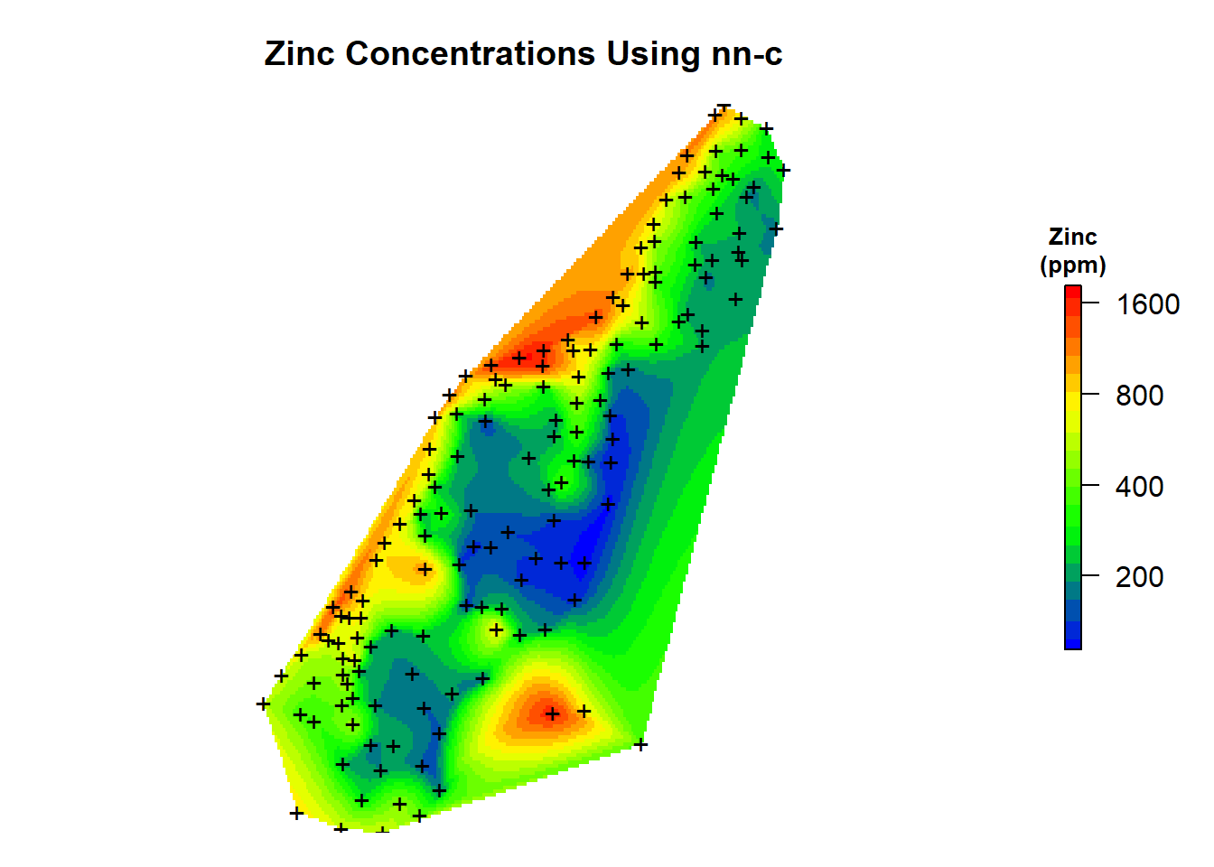
Natural Neighbor Interpolation Using nn-c
One of the drawbacks of Sibson’s original algorithm was the large computational overhead required to perform an interpolation. The operation required modifying the Voronoi diagram to introduce a new polygon, and then removing that polygon when the interpolation was complete. This can be computationally costly, especially when the number of grid cells is large. An alternative approach for streamlining the interpolation is by replacing the Voronoi diagram with a related structure, the Delaunay triangulation (Watson 1981). Delaunay triangulation and the Voronoi diagram are dual graphs of each other, meaning that any set of sample points that produces a unique Delaunay triangulation will also produce a corresponding unique Voronoi diagram. Once the initial Delaunay triangulation is established, the triangulation can be used to perform as many interpolations as desired without ever needing to modify the underlying structure. This approach eliminates a the computational overhead of directly using Voronoi polygons and expedites the interpolation process. The number of natural neighbors is determined by constructing natural neighbor circles, called circumcircles. Two points are natural neighbors if they lie on the same natural neighbor circle. Delaunay triangulation is then used to determine the weights for interpolation.
nn is a C code for natural neighbor interpolation of 2D scattered data. It provides a C library and a command line utility nnbathy. Algorithmically, it was initially loosely based on nngridr (Watson 1994), but code-wise, it is an independent development. nn is coded for robustness (to handle degenerate data) and scalability (to handle millions of data points), subject to using double precision calculations. For the underlying Delaunay triangulation it calls exact arithmetic code from Triangle, developed by Jonathan Richard Shewchuk.
The nn code was developed on a pc-linux platform, however, it can be compiled on other platforms. One note of caution is that the code in triangle.c assumes the triangles are four-byte-aligned and that “unsigned long” type is adequate to hold a pointer. Unsigned long did not work as a pointer in x64 so I changed it to “unsigned long long”.
The command line utility nnbathy uses a three-column file with points to interpolate from (actual observation file) and a two-column file with points to interpolate to (grid file). Let’s create these files and sve them to the data file within the working directory.
# Get locations
myvars <- c('x', 'y', 'zinc')
dat <- meuse[, myvars]

# Save data
fname <- './data/meuse_zinc.txt'
write.table(dat, file = fname, sep = " ",
  row.names = F, col.names = F, append = F)

# Save grid
fname <- './data/grid.txt'
write.table(grid2D$grid, file = fname, sep = " ",
  row.names = F, col.names = F, append = F)
Let’s use system2 in base R to invoke the OS command to run nnbathy.
# Setup variables
cmd_name <- "C:/cholbert/__temp/natural_neighbor/compile/nn/nnbathy.exe"
param1 <- "-i meuse_zinc.txt"
param1 <- "-i ./data/meuse_zinc.txt"
param2 <- "-o ./data/grid.txt"

# Call nnbathy and run interpolation
system2(cmd_name, args = c(param1, param2), stdout = "./data/nnbathy_results.txt")
Now, let’s read the saved results of the interpolation.
# Load nnbathy results
zn.nnbathy <- read.table('data/nnbathy_results.txt', header = FALSE) %>%
  rename(x = V1, y = V2, pred = V3)
Now, let’s add the predictions to our spatial pixels object and create a map of the natural neighbor predictions that were made using the nn C code.
# Add predictions to spatial pixels object
meusegrid.spdf$zn.nnbathy <- zn.nnbathy$pred

# Create plot
par(mar = c(1, 1, 3, 2))  # bottom, left, top, right; default is c(5.1, 4.1, 4.1, 2.1)
plot(
  log10(raster(meusegrid.spdf['zn.nnbathy'])),
  col = leg,
  main = "Zinc Concentrations Using nn-c",
  axes = FALSE,
  box = FALSE,
  axis.args = axis.ls,
  legend.args = list(text = "Zinc\n(ppm)", side = 3, font = 2, line = 0.2, cex = 0.8)
)
points(coordinates(meuse.spdf), pch = "+")
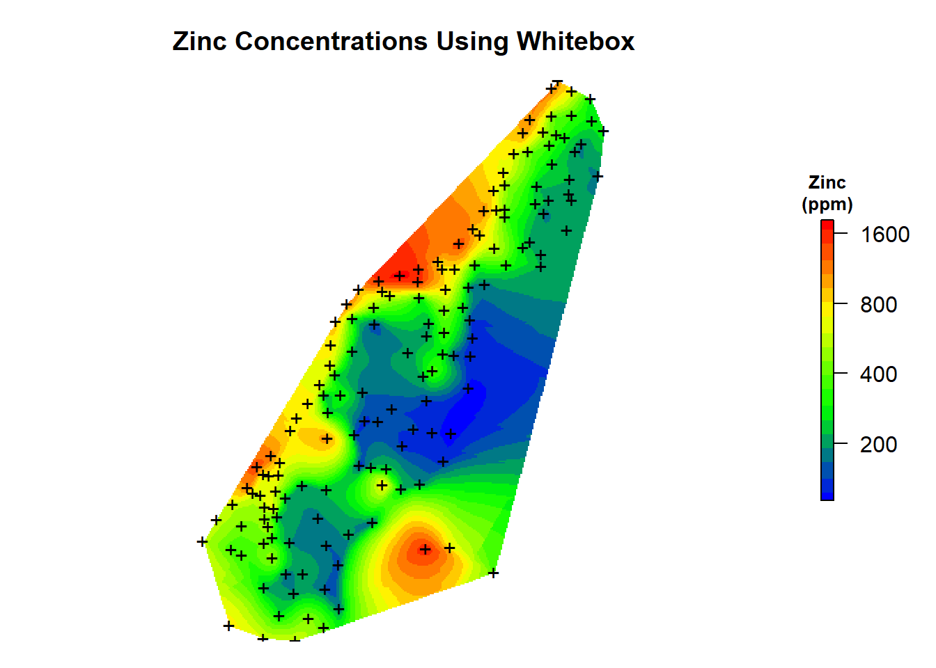
Natural Neighbor Interpolation Using Whitebox
The R whitebox library is a frontend for a stand-alone executable command-line program called WhiteboxTools, which is an advanced geospatial data analysis platform developed by Prof. John Lindsay at the University of Guelph’s Geomorphometry and Hydrogeomatics Research Group. WhiteboxTools can be used to perform common geographical information systems (GIS) analysis operations, remote sensing and image processing tasks, spatial hydrological analysis, terrain analysis, and LiDAR data processing.
First, let’s save the meuse spatial points data frame as a shape file.
# Save shapefile
f1 <- paste0(getwd(), '/shapes/', 'meuse.shp')
raster::shapefile(meuse.spdf, f1)
Now, let’s use the wbt_natural_neighbour_interpolation() function to interpolate the set of input vector points from the shape file onto a raster grid using Sibson’s (1981) natural neighbor method.
# Load library
library(whitebox)

# Run natural neighbor interpolation
wbt_natural_neighbour_interpolation(
  input = './shapes/meuse.shp',
  output = './data/meuse_zinc.tif',
  field = 'zinc',
  use_z = FALSE,
  cell_size = 10,
  base = NULL,
  clip = TRUE,
  wd = getwd(),
  verbose_mode = FALSE,
  compress_rasters = FALSE,
  command_only = FALSE
)
Finally, let’s load the raster grid and create a map of the natural neighbor predictions that were made using the whitebox library.
# Load interpolation results
zn.wb <- raster('data/meuse_zinc.tif')

# Create plot
par(mar = c(1, 1, 3, 2))  # bottom, left, top, right; default is c(5.1, 4.1, 4.1, 2.1)
plot(
  log10(zn.wb),
  col = leg,
  main = 'Zinc Concentrations Using Whitebox',
  axes = FALSE,
  box = FALSE,
  axis.args = axis.ls,
  legend.args = list(text = "Zinc\n(ppm)", side = 3, font = 2, line = 0.2, cex = 0.8)
)
points(coordinates(meuse.spdf), pch = "+")
References
Goovaerts, P. 1997. Geostatistics for Natural Resource Evaluation. Oxford University Press, New York.
Isaaks, E.H. and R.M. Srivastava. 1989. An Introduction to Applied Geostatistics. Oxford University Press. New York.
Sibson, R. 1981. A Brief Description of Natural Neighbor Interpolation. In Interpolating Multivariate Data. John Wiley & Sons, New York, pp. 21-36.
Watson, D. F. 1981. Computing the n-dimensional Delaunay tessellation with application to Voronoi polytropes. The Computer Journal 24, pp. 167-173.
Watson, D.F. 1994. Nngridr: An Implementation of Natural Neighbor Interpolation. Claremont, Australia.
- Posted on:
- May 22, 2023
- Length:
- 18 minute read, 3816 words
- See Also: