Introduction

The 95 percent upper confidence limit of the mean (95% UCL or UCL95) is a frequently used statistical measure in environmental sciences. For example, when compliance point data are to be compared to a fixed standard and the standard represents an average or true mean concentration, a confidence interval around the mean is the method of statistical choice. A confidence interval around the mean is designed to estimate the true average of the underlying population, while at the same time accounting for variability in the sample data. For a collection of samples, the UCL95 is defined as a value that equals or exceeds the actual average of a distribution 95 percent of the time. In most cases, as the number of samples increase, the UCL95 will decrease and approach the true mean concentration. For small sample sizes (less than 8), any method used for computing the UCL95 is based on sufficiently few observations that the estimate is likely to be highly uncertain. The lower bound of 8 observations is based on simulations in determining the distributional shape of the data. Below eight, there’s insufficient data to even guess what the distributional shape may be. Small sample sizes also provide poor estimates of the mean of the data. With larger data sets (20 observations or more), bootstrapping can be used to provide a good estimate of the mean regardless of the shape of the data.

For a given data set, there are a number of different methods for calculating a UCL95. The preferred approach depends on many factors, including the number of samples, the distribution of the data, and whether the data include non-detect observations. The purpose of this blog post is to present and demonstrate the basic methods for computing a UCL95 on the mean of an unknown population for left-censored data sets (i.e., containing a mixture of detects and non-detects) using the R language for statistical computing and visualization.

Managing Non-Detects

For data sets consisting of non-detects with multiple censoring limits, several estimation methods are available, including maximum likelihood estimation (MLE), Kaplan-Meier (KM) product-limit estimator (Kaplan and Meier 1958), and robust regression on order statistics (rROS) (Helsel 2012). A brief description of each of these methods is provided below. Additional information can be found in USEPA (2015), Helsel (2012), and Singh et al. (2006).

The MLE method assumes that data have a particular shape (or distribution). The method fits a distribution to the data that matches both the values for detected observations, and the proportion of observations falling below each detection limit. The information contained in non-detects is captured by the proportion of data falling below each detection limit. Because the model uses the parameters of a probability distribution, MLE is a fully parametric approach and all inference is based on the assumed distribution. A limitation of MLE is that the appropriate probability distribution to which the data belong must be specified, and the data sample size should be large enough to enable verification that the assumed data distribution is reasonable.

The rROS method is semi-parametric in the sense that part of the inference is based on an assumed distribution and part of the inference is based on the observed values, without any distributional assumption. Unlike Kaplan-Meier, ROS internally assumes that the underlying population is approximately normal or lognormal. However, the assumption is directly applied to only the censored measurements and not to the full data set. In particular, ROS plots the detected values on a probability plot (with a regular or log-transformed axis) and calculates a linear regression line in order to approximate the parameters of the underlying (assumed) distribution. This fitted distribution is then utilized to generate imputed estimates for each of the censored measurements, which are then combined with the known (detected) values to compute summary statistics of interest (e.g., mean, variance). The method is labeled “robust” because the detected measurements are used “as is” to make estimates, rather than simply using the fitted distributional parameters from the probability plot.

The KM method is a standard nonparametric method for computing descriptive statistics of censored data. It is widely used in survival or lifetime data analysis to incorporate data with multiple censoring levels and does not require specification of an assumed distribution. A percentile is assigned to each detected observation, starting at the largest detected value and working down the data set, based on the number of detects and nondetects above and below each observation. Percentiles are not assigned to nondetects, but nondetects affect the percentiles calculated for detected observations. The survival curve, a step function plot of the cumulative distribution function, gives the shape of the data set. Estimates of the mean and standard deviation are computed from the estimated cumulative distribution function and these estimates then can be used in parametric statistical tests.

Load Libraries

We’ll start by loading the required R libraries. The main R library that we will be using for the computations is the EnvStats library. The EnvStats library includes methods for the graphical and statistical analyses of environmental data, with a focus on analyzing chemical concentrations and physical parameters, usually in the context of mandated environmental monitoring.

# Load libraries
library(dplyr)
library(EnvStats)
library(bootstrap)

Data

Let’s load the data. The data are comprised of cadmium concentrations in 32 surface soil samples with a mixture of detects and non-detects. There are six variables in the data set, including sample id, analytical method, parameter name, a detected field, results, and units.

# Read data in comma-delimited file
datin <- read.csv('data/cadmium.csv', header = T)

# Inspect structure of the data
str(datin)
## 'data.frame':	32 obs. of  6 variables:
##  $ Sample  : chr  "S1018" "S1019" "S1020" "S1021" ...
##  $ Method  : chr  "SW6020" "SW6020" "SW6020" "SW6020" ...
##  $ Param   : chr  "Cadmium" "Cadmium" "Cadmium" "Cadmium" ...
##  $ Detected: chr  "Y" "Y" "Y" "Y" ...
##  $ Result  : num  1.87 1.8 1.73 1.72 0.4 1.2 1.06 2 0.8 0.92 ...
##  $ Units   : chr  "mg/kg" "mg/kg" "mg/kg" "mg/kg" ...

Let’s add a variable to the data that identifies whether the result is censored (non-detect) or is not censored (detect). This field is generally required for most of the methods used for analyzing censored data sets.

# Prep data
dat <- datin %>%
  mutate(
    Censored = ifelse(Detected == 'N', TRUE, FALSE)
  ) %>%
  data.frame()

Descriptive Statistics

Let’s create a function to calculate descriptive statistics, including the total number of samples, the number of detected results, and the frequency of detection; the minimum and maximum concentrations for detected and non-detected observations; and the mean, median, standard deviation, and coefficient of variation (CV). The mean and median provide a measure of central tendency, while the standard deviation and CV provide a measure of variability in the data. The CV is the ratio of the sample standard deviation to the sample mean and thus indicates whether the amount of “spread” in the data is small or large relative to the average observed magnitude. Values less than one indicate that the standard deviation is smaller than the mean, while values greater than one occur when the standard deviation is greater than the mean.

For this example, the KM product-limit estimator will be used to compute the descriptive statistics with the censoring limit set at the detection limit. If a data set is a mixture of detects and non-detects, but the non-detect fraction is no more than 50 percent, a censored estimation method such as the KM product-limit estimator or rROS can be used to compute adjusted estimates of the mean and standard deviation. Because parameter estimation can suffer for data sets with low detection frequencies, the USEPA (2009) recommends that these methods should not be used when more than 50 percent of the data are non-detects.

# Function to compute summary statistics
sumstats <- function(dd, rv = 3, trans = TRUE) {
  cdat <- dd %>%
    group_by(Param) %>%
    summarize(
      Obs     = length(Result),
      Dets    = length(Result[!Censored]),
      DetFreq = round(Dets * 100 / Obs, 2),
      MinND   = tryCatch(
        min(Result[Censored], na.rm = T),
        warning = function(e) NA
      ),
      MinDET  = tryCatch(
        min(Result[!Censored], na.rm = T),
        warning = function(e) NA
      ),
      MaxND   = tryCatch(
        max(Result[Censored], na.rm = T),
        warning = function(e) NA
      ),
      MaxDet  = tryCatch(
        max(Result[!Censored], na.rm = T),
        warning = function(e) NA
      ),
      Mean = tryCatch(
        enparCensored(Result, Censored)$parameters['mean'],
        error = function(e) mean(Result, na.rm = T)
      ),
      Median = tryCatch(
        median(
          ppointsCensored(Result, Censored,
          prob.method = 'kaplan-meier'
        )$Order.Statistics),
        error = function(e) median(Result, na.rm = T)
      ),
      SD = tryCatch(
        enparCensored(Result, Censored)$parameters['sd'],
        error = function(e) sd(Result, na.rm = T)
      ),
      CV = tryCatch(SD / Mean, error = function(e) NA),
    .groups = 'drop') %>%
    mutate(across(where(is.numeric), \(x) round(x, rv))) %>%
    data.frame()

  # Change values if less than 50% detections
  cdat$Mean[cdat$DetFreq < 50] <- NA
  cdat$Median[cdat$DetFreq < 50] <- NA
  cdat$SD[cdat$DetFreq < 50] <- NA
  cdat$CV[cdat$DetFreq < 50] <- NA

  # Transpose summary statistics
  if (trans) {
    names <-  cdat[,1]              # keep 1st column
    cdat.T <- as.data.frame(as.matrix(t(cdat[,-1])))  # transpose everything but 1st column
    colnames(cdat.T) <- names       # assign 1st column as column names
    cdat <- cdat.T
  }
  return(cdat)
}

Now, let’s compute the descriptive statistics for our cadmium data.

# Get summary statistics
sumstats(dat)
##         Cadmium
## Obs      32.000
## Dets     24.000
## DetFreq  75.000
## MinND     0.400
## MinDET    0.440
## MaxND     1.100
## MaxDet    2.900
## Mean      1.257
## Median    1.100
## SD        0.697
## CV        0.554

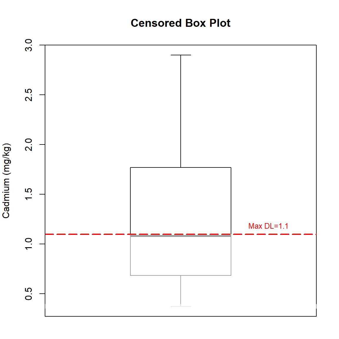
Concentrations range from <0.4 to 2.9 milligrams-per kilogram (mg/kg) with a mean concentration of 1.26 mg/kg and a median concentration of 1.1 mg/kg. The standard deviation is 0.697 mg/kg and the CV is 0.554.

Graphical Presentations of the Data

Let’s use the NADA2 library to create a censored box plot of the data. The highest censoring limit is shown as the red, dashed horizontal line. Any statistics below this line must be estimated using methods for censored data.

# Create censored boxplot using NADA2 package
library(NADA2)
par(mar=c(2,4,4,2))
with(dat, cboxplot(
  x1 = Result, x2 = Censored,
  LOG = FALSE,
  show = TRUE,
  Ylab = 'Cadmium (mg/kg)',
  Title = 'Censored Box Plot',
  minmax = TRUE,
  printstat = TRUE
  )
)
##   MaximumDL Group
## 1       1.1   all

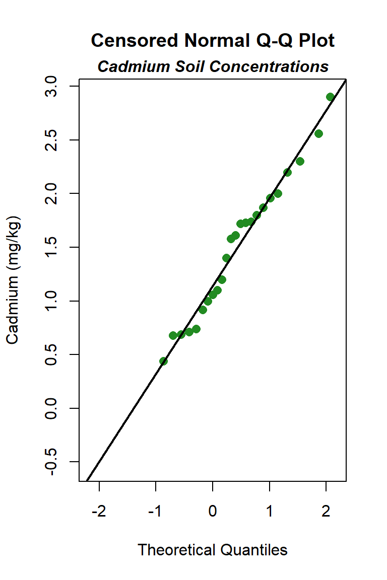
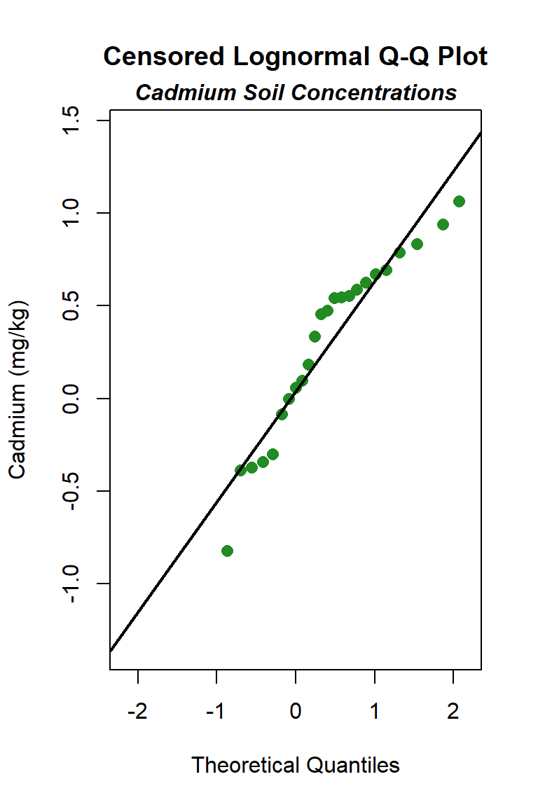
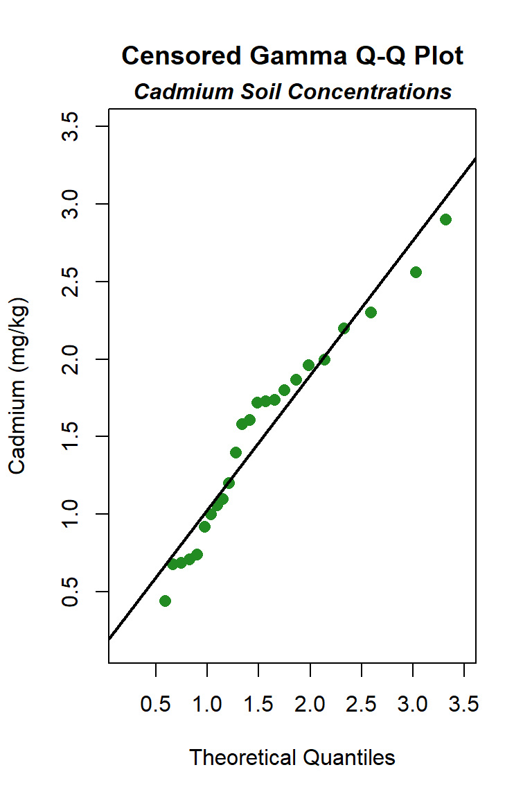
Let’s create quantile-quantile (Q-Q) plots showing the ordered sample results versus the corresponding quantiles of a normal, lognormal, and gamma data distribution. Because quantiles are associated with cumulative probabilities, Q-Q plots are also referred to as probability plots. A normal probability plot is used to evaluate the normality of the distribution of a variable (that is, whether, and to what extent, the distribution of the variable follows the normal distribution). If the data are not normally distributed, they will deviate systematically from a straight line. Variability in the data will cause the data to scatter randomly around this line but the data will still appear to follow a single straight line. In addition to providing information about the data distributions, Q-Q plots are useful in identifying outliers potentially present in a data set. On a Q-Q plot, observations well-separated from the majority of the data may represent potential outliers coming from a population different from the main sample population.

# Function to create Q-Q plot
get_qqplot <- function(x, xcen, dist = 'norm') {
  if (dist == 'gamma') {
    qqPlotCensored(
      x, xcen,
      distribution = dist,
      estimate.params = TRUE,
      prob.method = 'modified kaplan-meier',
      pch = 16, cex = 1.2, points.col = 'forestgreen',
      add.line = TRUE, line.lwd = 2,
      xlab = 'Theoretical Quantiles',
      ylab = 'Cadmium (mg/kg)',
      font.lab = 1, cex.lab = 1, cex.axis = 1,
      cex.main = 1.2,
      main = 'Censored Gamma Q-Q Plot'
    )
    mtext(
      'Cadmium Soil Concentrations',
      side = 3, line = 0.2, font = 4, cex = 1
    )
  } else {
    if (dist == 'norm') main_title <- 'Censored Normal Q-Q Plot'
    if (dist == 'lnorm') main_title <- 'Censored Lognormal Q-Q Plot'
    qqPlotCensored(
      x, xcen,
      distribution = dist,
      prob.method = 'modified kaplan-meier',
      pch = 16, cex = 1.2, points.col = 'forestgreen',
      add.line = TRUE, line.lwd = 2,
      xlab = 'Theoretical Quantiles',
      ylab = 'Cadmium (mg/kg)',
      font.lab = 1, cex.lab = 1, cex.axis = 1,
      cex.main = 1.2,
      main = main_title
    )
    mtext(
      'Cadmium Soil Concentrations',
      side = 3, line = 0.2, font = 4, cex = 1
    )
  }
}

# Create Q-Q plots for each distribution
with(dat, get_qqplot(x = Result, xcen = Censored, dist = 'norm'))
with(dat, get_qqplot(x = Result, xcen = Censored, dist = 'lnorm'))
with(dat, get_qqplot(x = Result, xcen = Censored, dist = 'gamma'))

Goodness-of-fit Test

Let’s create a functon to perform a probability plot correlation coefficient (PPCC) goodness-of-fit test to determine whether the censored cadmium data appear to come from a normal distribution, lognormal distribution, or gamma distribution. The PPCC test measures and evaluates the linearity of the probability plot. The square of this statistic is equivalent to the Weisberg-Bingham Approximation to the Shapiro-Francia W’-test (Weisberg and Bingham 1975; Royston 1993). Thus, the PPCC goodness-of-fit test is equivalent to the Shapiro-Francia goodness-of-fit test.

# Function to get gof statistics
gof_test <- function(x, xcen, dist = 'norm') {
  gofTestCensored(
    x, xcen,
    censoring.side = 'left',
    test = 'ppcc',
    distribution = dist,
    prob.method = 'hirsch-stedinger'
  )
}

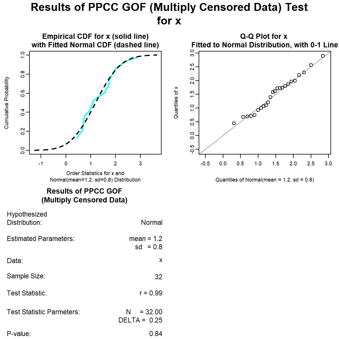
Let’s perform a goodness-of-fit test for a normal distribution.

norm.gof <- with(dat, gof_test(Result, Censored, dist = 'norm'))
plot(norm.gof)

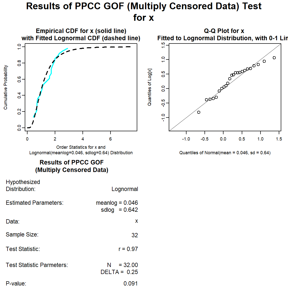
Let’s perform a goodness-of-fit test for a lognormal distribution.

lnorm.gof <- with(dat, gof_test(Result, Censored, dist = 'lnorm'))
plot(lnorm.gof)

Let’s perform a goodness-of-fit test for a gamma distribution.

gamma.gof <- with(dat, gof_test(Result, Censored, dist = 'gamma'))
plot(gamma.gof)

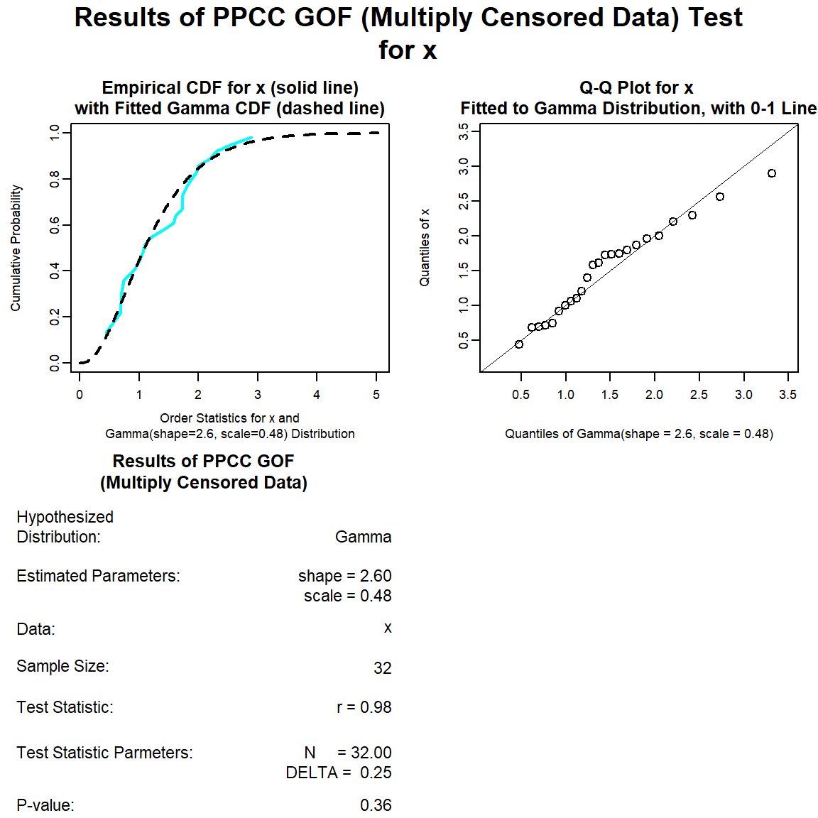
The distribution with the highest (closest to 1) PPCC is the normal distribution, followed by the gamma distribution and then the lognromal distribution.

We also can use the distChooseCensored() function to perform a series of goodness-of-fit tests for censored data from a set of candidate probability distributions to determine which probability distribution provides the best fit for a data set. By setting the method = “proucl”, the distChooseCensored() function uses the algorithm from USEPA’s ProUCL software (USEPA 2015) to determine the best fitting distribution. The candidate distributions are the normal, lognormal, and gamma distributions.

# Perform a series of goodness-of-fit tests for censored data using
# distChooseCensored() function and ProUCL method.
all.gof <- with(dat,
  distChooseCensored(
    Result, Censored,
    method = 'proucl',
    choices = c('norm', 'gammaAlt', 'lnormAlt'),
    keep.data = FALSE
  )
)
all.gof$decision
## [1] "Normal"

Based on the ProUCL algorithm, the data can be assumed to follow a normal distribution.

UCL95 Calculations

Let’s create some functions for computing the UCL95 assuming different distributions and for data with and without non-detects. First, let’s create a function for computing the UCL95 assuming a normal distribution. We’ll use the KM product-limit estimator as the default method for data containing non-detects.

# Function for normal UCL
ucl_norm <- function(x, cen, method = 'KM') {
  if (sum(cen) == 0) {
    ucl <- enorm(
      x, method = 'mvue',
      ci = TRUE, ci.type = 'upper', conf.level = 0.95,
      ci.method = 'exact'
    )$interval$limits[['UCL']]
  } else if (method == 'KM') {
    n <- length(x)
    m <- enparCensored(x, cen)$parameters[['mean']]
    s <- enparCensored(x, cen)$parameters[['sd']]
    se <- enparCensored(x, cen)$parameters[['se.mean']]
    ucl <- m + qt(0.95, n-1)*s/sqrt(n)
  } else {
    ucl <- enormCensored(
      x, cen, method = 'rROS',
      ci = TRUE, ci.type = 'upper', conf.level = 0.95,
      ci.method = 'bootstrap', n.bootstraps = 1000,
      lb.impute = 0.1 * min(x[cen]),
      ub.impute = max(x[cen])
    )$interval$limits[['BCa.UCL']]
  }
  return(ucl)
}

Second, let’s create a function for computing the UCL95 assuming a lognormal distribution. We’ll use rROS as the default method for data containing non-detects.

# Function for lognormal UCL
ucl_lnorm <- function(x, cen, method = 'rROS') {
  if (sum(cen) == 0) {
    ucl <- elnormAlt(
      x, method = 'mvue',
      ci = TRUE, ci.type = 'upper', conf.level = 0.95,
      ci.method = 'cox'
    )$interval$limits[['UCL']]
  } else if (method == 'rROS') {
    ucl <- elnormAltCensored(
      x, cen, method = 'rROS',
      ci = TRUE, ci.type = 'upper', conf.level = 0.95,
      ci.method = 'bootstrap', n.bootstraps = 1000
    )$interval$limits[['BCa.UCL']]
  } else if (method == 'KM') {
    n <- length(x)
    mx <- roundUp(1/min(x) + 1)
    kmlog <- enparCensored(log(x * mx), cen, ci = FALSE)
    mean.kmlog <- kmlog$parameters[['mean']] - log(mx)
    sd.kmlog <- kmlog$parameters[['sd']]
    m <- exp(mean.kmlog + 0.5 * sd.kmlog^2)
    s <- sqrt(exp(2 * mean.kmlog + sd.kmlog^2) * (exp(sd.kmlog^2) - 1))
    ucl <- m + qt(0.95, n-1)*s/sqrt(n)
  } else {
    ucl <- elnormAltCensored(
      x, cen, method = 'mle',
      ci = TRUE, ci.type = 'upper', conf.level = 0.95,
      ci.method = 'bootstrap', n.bootstraps = 1000
    )$interval$limits[['BCa.UCL']]
  }
  return(ucl)
}

Third, let’s create a function for computing the UCL95 assuming a gamma distribution. We’ll use the KM product-limit estimator as the default method for data containing non-detects.

# Function for gamma UCL
ucl_gamma <- function(x, cen, method = 'KM') {
  if (sum(cen) == 0) {
    ucl <- egammaAlt(
      x, method = 'mle',
      ci = TRUE, ci.type = 'upper', conf.level = 0.95,
      ci.method = 'normal.approx',
      normal.approx.transform = 'kulkarni.powar'
    )$interval$limits[['UCL']]
  } else if (method == 'KM') {
    n <- length(x)
    m <- enparCensored(x, cen)$parameters[['mean']]
    s <- enparCensored(x, cen)$parameters[['sd']]
    k <- (m/s)^2
    kstar <- (n - 3) * k / n + 2 /(3*n)
    qchisq(0.05, df = 2*n*kstar)
    ucl <- 2 * n * kstar * m / qchisq(0.05, df = 2*n*kstar)
  } else {
    ucl <- egammaAltCensored(
      x, cen, method = 'mle',
      ci = TRUE, ci.type = 'upper', conf.level = 0.95,
      ci.method = 'bootstrap', n.bootstraps = 1000
    )$interval$limits[['BCa.UCL']]
  }
  return(ucl)
}

Finally, let’s create a function for computing the UCL95 assuming no distribution. We’ll use the KM product-limit estimator as the default method for data containing non-detects.

# Function for nonparametric UCL
ucl_nonpar <- function(x, cen) {
  if (sum(cen) == 0) {
    meanfun <- function (d, i) {
      x <- d[i]
      mean(x)
    }
    bmean <- boot(data = x, statistic = meanfun, R = 1000)
    ucl <- boot.ci(bmean, conf = 0.90, type = 'perc')$percent[[5]]
  } else {
    ucl <- enparCensored(
      x, cen,
      ci = TRUE, ci.type = 'upper', conf.level = 0.95,
      ci.method = 'bootstrap', n.bootstraps = 1000
    )$interval$limits[['BCa.UCL']]
  }
  return(ucl)
}

Now, let’s compute the UCL95 for the cadmium data using all of the methods.

# Set seed
set.seed(1515)

ucl.norm  <- with(dat, ucl_norm(Result, Censored))
ucl.gamma <- with(dat, ucl_gamma(Result, Censored))
ucl.lnorm <- with(dat, ucl_lnorm(Result, Censored))
ucl.npar <- with(dat, ucl_nonpar(Result, Censored))

# Compare results
data.frame(
  normal = ucl.norm,
  lognormal = ucl.lnorm,
  gamma = ucl.gamma,
  nonpar = ucl.npar
) %>% round(2)
##   normal lognormal gamma nonpar
## 1   1.47      1.46   1.5   1.46

For this data set, the results are remarkably similar. The UCL95 of the mean cadmium concentration ranges from 1.46 mg/kg, assuming a lognormal distribution, to 1.50 mg/kg for a gamma distribution. Assuming a normal distribution, the UCL95 is 1.47 mg/kg. The nonparametric bootstrap UCL95 is 1.46 mg/kg.

Although the goodness-of-fit tests indicate the cadmium data can be assumed to follow a normal distribution, a concern of the normal distribution is that it may allow the lower end of the distribution to go negative, an unrealistic situation for environmental variables that produces an estimate of the mean, and perhaps the UCL. To test this, we can use the estimates of the mean and standard deviation for the assumed normal distribution to compute whether 3 standard deviations below the mean is a negative number. If so, the lower end is indeed unrealistic. The fitted normal to these data indicates a mean of 1.257 mg/kg and a standard deviation of 0.697 mg/kg, which gives 1.257 - (3*0.697) = -0.834 mg/kg. The low end of the distribution is indeed described as below zero. This also is apparent in the normal Q-Q plot, which shows that the normal distribution line falls below a cadmium concentration of zero when the “quantiles of normal” is approximately -1.4. In this situation, in would be better to select the distribution with the next highest PPCC statistic for the UCL95 calculation, which here is the gamma distribution.

As a final note, environmental data are frequently right-skewed, and right-skewed data often follow a lognormal distribution. However, use of a parametric lognormal distribution on a lognormally distributed data set may yield unrealistically large upper limits, especially when the standard deviation of the log-transformed data becomes greater than 1 for small data sets (less than 30 to 50 measurements). Because environmental data typically can be modeled by a gamma distribution, gamma distribution limits generally are given preference over lognormal distribution limits, where appropriate.

References

Helsel, D.R. 2012. Statistics for Censored Environmental Data Using Minitab and R, Second Edition. John Wiley and Sons, NJ.

Kaplan, E.L. and O. Meier. 1958. Nonparametric Estimation from Incomplete Observations. JASA 53, 457-481.

Royston, P. 1993. A Toolkit for Testing for Non-Normality in Complete and Censored Samples. The Statistician 42, 37-43.

Singh, A., R. Maichle, and S. Lee. 2006. On the Computation of a 95% Upper Confidence Limit of the Unknown Population Mean Based Upon Data Sets with Below Detection Limit Observations. EPA/600/R-06/022, March.

United States Environmental Protection Agency (USEPA). 2009. Statistical Analysis of Groundwater Monitoring Data at RCRA Facilities: Unified Guidance. EPA-530-R-09-007. Office of Resource Conservation and Recovery, U.S. Environmental Protection Agency. March.

United States Environmental Protection Agency (USEPA). 2015. ProUCL Version 5.1 Technical Guide Statistical Software for Environmental Applications for Data Sets with and without Nondetect Observations. EPA/600/R-07/041. Office of Research and Development, U.S. Environmental Protection Agency. October.

Weisberg, S. and C. Bingham. 1975. An Approximate Analysis of Variance Test for Non-Normality Suitable for Machine Calculation. Technometrics 17, 133-134.